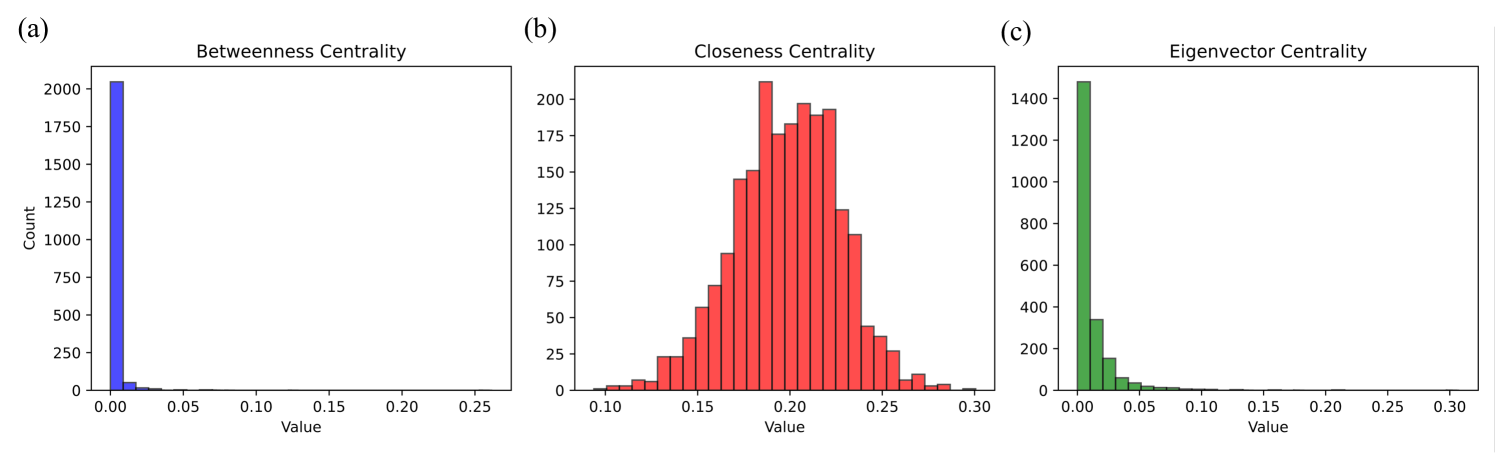
## Histogram: Network Centrality Metrics ### Overview The image presents three side-by-side histograms labeled (a), (b), and (c). These charts visualize the frequency distribution of three distinct centrality metrics—Betweenness, Closeness, and Eigenvector—calculated for nodes within a specific network. Each chart uses a different color scheme and axis scale to represent the distribution of values. ### Components/Axes **Chart (a): Betweenness Centrality** * **Position:** Leftmost panel. * **Color:** Blue bars. * **Y-Axis:** "Count", ranging from 0 to 2000, with increments of 250. * **X-Axis:** "Value", ranging from 0.00 to 0.25, with increments of 0.05. **Chart (b): Closeness Centrality** * **Position:** Center panel. * **Color:** Red bars. * **Y-Axis:** "Count", ranging from 0 to 200, with increments of 25. * **X-Axis:** "Value", ranging from 0.10 to 0.30, with increments of 0.05. **Chart (c): Eigenvector Centrality** * **Position:** Rightmost panel. * **Color:** Green bars. * **Y-Axis:** "Count", ranging from 0 to 1400, with increments of 200. * **X-Axis:** "Value", ranging from 0.00 to 0.30, with increments of 0.05. ### Detailed Analysis **Chart (a) - Betweenness Centrality (Blue)** * **Trend:** The distribution is heavily right-skewed (positive skew). The vast majority of the data is concentrated at the lowest possible value (0.00). * **Data Points:** The peak bar at 0.00 exceeds a count of 2000. The frequency drops sharply immediately after 0.00, with a very small "tail" extending toward 0.05. There is negligible data beyond 0.05. **Chart (b) - Closeness Centrality (Red)** * **Trend:** The distribution follows a roughly normal (bell-shaped) curve. * **Data Points:** The distribution is centered around 0.20. The peak count is slightly above 200. The data is spread across the range of 0.10 to 0.30, with the frequency tapering off symmetrically on both sides of the 0.20 center point. **Chart (c) - Eigenvector Centrality (Green)** * **Trend:** Similar to chart (a), this distribution is heavily right-skewed. * **Data Points:** The peak bar is at 0.00, with a count approaching 1500. The frequency decreases rapidly as the value increases. There is a visible, thin tail extending out to approximately 0.10, with almost zero frequency beyond 0.15. ### Key Observations * **Distribution Contrast:** Charts (a) and (c) exhibit power-law-like distributions, where the overwhelming majority of nodes have near-zero centrality, while chart (b) exhibits a normal distribution. * **Scale Variance:** The Y-axis scales differ significantly, indicating that the total number of nodes or the density of the network is represented differently across these metrics, or that the metrics themselves have vastly different ranges of output. * **Outliers:** In charts (a) and (c), the "tail" represents the few nodes that possess high centrality, acting as potential hubs or bridges within the network. ### Interpretation The data suggests this network possesses characteristics typical of real-world complex networks (such as social networks, biological networks, or the internet). * **Betweenness and Eigenvector Centrality:** The heavy skew toward zero indicates that most nodes in this network are peripheral or "leaf" nodes. They do not act as significant bridges between other nodes (low betweenness) and are not connected to other highly influential nodes (low eigenvector centrality). Only a very small fraction of nodes act as "hubs" or critical connectors. * **Closeness Centrality:** The normal distribution centered around 0.20 suggests that, despite the hierarchical nature implied by the other two metrics, the network maintains a "small-world" property. Most nodes are at a relatively similar average distance from all other nodes in the network, suggesting a cohesive structure where information or influence can propagate relatively efficiently, even if most nodes are not "hubs." * **Synthesis:** This combination of metrics describes a network with a core-periphery structure: a few highly central nodes (the tail in a and c) exist within a larger, relatively uniform background of nodes that are all roughly equidistant from one another (the bell curve in b).