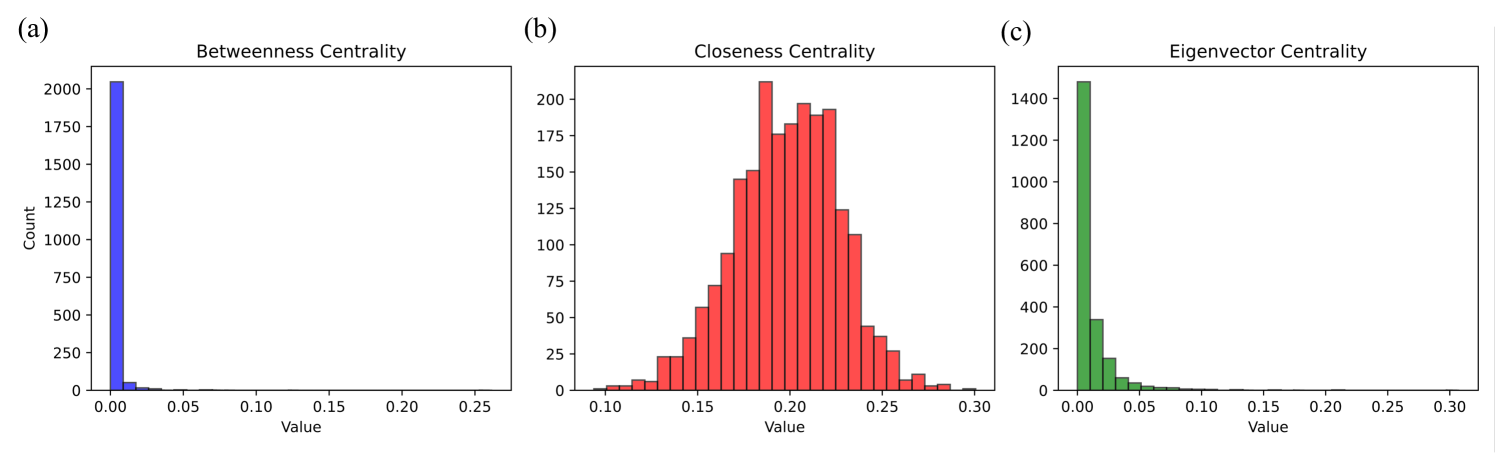
\n ## Histograms: Network Centrality Measures ### Overview The image presents three histograms, each representing the distribution of a different network centrality measure: Betweenness Centrality, Closeness Centrality, and Eigenvector Centrality. Each histogram displays the 'Value' of the centrality measure on the x-axis and the 'Count' (frequency) on the y-axis. The histograms are labeled (a), (b), and (c) respectively. ### Components/Axes * **X-axis (all histograms):** Labeled "Value". The scale ranges from 0.00 to 0.30, with increments of 0.05. * **Y-axis (all histograms):** Labeled "Count". The scale varies for each histogram. * **(a) Betweenness Centrality:** Histogram is filled with a blue color. Y-axis ranges from 0 to 2000, with increments of 250. * **(b) Closeness Centrality:** Histogram is filled with a red color. Y-axis ranges from 0 to 200, with increments of 25. * **(c) Eigenvector Centrality:** Histogram is filled with a red color. Y-axis ranges from 0 to 1400, with increments of 200. ### Detailed Analysis or Content Details **(a) Betweenness Centrality:** The distribution is heavily skewed to the left. The vast majority of nodes have a Betweenness Centrality value close to 0. The histogram shows a peak around a value of approximately 0.00, with a count of around 1800. The count rapidly decreases as the value increases, with very few nodes having a Betweenness Centrality value greater than 0.05. **(b) Closeness Centrality:** The distribution is approximately normal, but slightly skewed to the right. The peak of the distribution is around a value of 0.18-0.20, with a count of approximately 180. The distribution extends to a value of approximately 0.30, with a decreasing count. **(c) Eigenvector Centrality:** The distribution is similar to Closeness Centrality, also approximately normal and slightly skewed to the right. The peak of the distribution is around a value of 0.16-0.18, with a count of approximately 1200. The distribution extends to a value of approximately 0.30, with a decreasing count. ### Key Observations * Betweenness Centrality has a very different distribution compared to Closeness and Eigenvector Centralities. It is highly concentrated near zero, indicating that most nodes have low Betweenness Centrality. * Closeness and Eigenvector Centralities have similar distributions, suggesting that nodes with high closeness tend to also have high eigenvector centrality, and vice versa. * The range of values for Betweenness Centrality is much smaller than for Closeness and Eigenvector Centralities. ### Interpretation These histograms provide insights into the structure of the network. The low Betweenness Centrality values for most nodes suggest that the network is not heavily reliant on a few nodes to act as bridges between different parts of the network. The distributions of Closeness and Eigenvector Centralities indicate that there are some nodes that are well-connected and influential within the network. The similarity between these two distributions suggests that the network's structure promotes both efficient communication (Closeness) and influence (Eigenvector). The differences in the distributions suggest that the network's structure is complex and that different centrality measures capture different aspects of the network's organization. The fact that the distributions are not perfectly normal suggests that the network is not a random graph and that its structure is influenced by specific factors.