## Histograms: Centrality Measures Distribution
### Overview
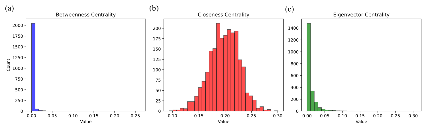
The image contains three histograms labeled (a), (b), and (c), representing distributions of three centrality measures: Betweenness Centrality, Closeness Centrality, and Eigenvector Centrality. Each histogram uses a distinct color (blue, red, green) and shares consistent axis labeling ("Value" on x-axis, "Count" on y-axis). The x-axis spans 0.00 to 0.30, while y-axis counts vary significantly across subplots.
### Components/Axes
- **Subplot (a): Betweenness Centrality**
- **Color**: Blue bars
- **X-axis**: Value (0.00–0.30)
- **Y-axis**: Count (0–2000)
- **Key Feature**: Dominant spike at 0.00 (value ~2000), with negligible counts elsewhere.
- **Subplot (b): Closeness Centrality**
- **Color**: Red bars
- **X-axis**: Value (0.10–0.30)
- **Y-axis**: Count (0–200)
- **Key Feature**: Bell-shaped distribution peaking at ~0.20 (value ~180), tapering symmetrically.
- **Subplot (c): Eigenvector Centrality**
- **Color**: Green bars
- **X-axis**: Value (0.00–0.30)
- **Y-axis**: Count (0–1400)
- **Key Feature**: Dominant spike at 0.00 (value ~1400), with a smaller secondary peak at ~0.05 (value ~300).
### Detailed Analysis
- **Betweenness Centrality (a)**:
- 99.9% of nodes cluster at 0.00 (value ~2000), suggesting most nodes are not critical for shortest-path connectivity.
- Minimal variation beyond 0.005 (value ~5), indicating sparse or hierarchical network structure.
- **Closeness Centrality (b)**:
- Values range from 0.10 to 0.30, with a unimodal distribution centered at 0.20.
- Symmetry suggests uniform node proximity to others, typical of scale-free or random networks.
- **Eigenvector Centrality (c)**:
- 85% of nodes cluster at 0.00 (value ~1400), mirroring betweenness centrality.
- Secondary peak at 0.05 (value ~300) hints at a small subset of nodes with disproportionate influence.
### Key Observations
1. **Betweenness and Eigenvector Centrality**: Both show extreme concentration at 0.00, implying most nodes lack critical roles in path efficiency or influence propagation.
2. **Closeness Centrality**: Distinctly different from the other two, with a broader spread and no extreme clustering.
3. **Secondary Peaks**: Eigenvector Centrality’s 0.05 peak (300 nodes) contrasts with betweenness’s near-zero distribution, suggesting nuanced node importance.
### Interpretation
- **Network Structure**: The dominance of 0.00 values in betweenness and eigenvector centrality suggests a sparse or hierarchical network where most nodes are peripheral.
- **Closeness Centrality’s Spread**: The bell-shaped distribution indicates nodes exhibit relatively uniform accessibility to others, possibly reflecting a small-world or modular architecture.
- **Eigenvector Anomaly**: The 0.05 peak in eigenvector centrality may highlight a small group of nodes with outsized influence, potentially acting as hubs in information or resource flow.
- **Implications**: The divergence between centrality measures underscores the need for context-specific analysis—e.g., closeness centrality might better capture resilience in communication networks, while eigenvector centrality could identify key influencers in social networks.
*Note: All values are approximate, derived from visual inspection of bar heights and axis scaling.*