## Scatter Plots: Test Loss vs. Compute, Dataset Size, and Parameters ### Overview The image presents three scatter plots illustrating the relationship between test loss and three different factors: compute (measured in PF-days, non-embedding), dataset size (measured in tokens), and parameters (non-embedding). Each plot shows a decreasing trend in test loss as the corresponding factor increases. ### Components/Axes **Plot 1: Test Loss vs. Compute** * **Y-axis:** Test Loss, linear scale from 2 to 7. * **X-axis:** Compute, logarithmic scale from 10^-9 to 10^1, labeled "PF-days, non-embedding". * **Data:** Multiple light blue lines, a black line representing an average, and a dashed orange line representing a fitted curve. * **Fitted Curve Equation (orange dashed line):** L = (Cmin / (2.3 * 10^8))^-0.050 **Plot 2: Test Loss vs. Dataset Size** * **Y-axis:** Test Loss, linear scale from 2.7 to 4.2. * **X-axis:** Dataset Size, logarithmic scale from 10^7 to 10^9, labeled "tokens". * **Data:** Blue data points connected by a blue line, and a gray fitted curve. * **Fitted Curve Equation (gray line):** L = (D / (5.4 * 10^13))^-0.095 **Plot 3: Test Loss vs. Parameters** * **Y-axis:** Test Loss, linear scale from 2.4 to 5.6. * **X-axis:** Parameters, logarithmic scale from 10^5 to 10^9, labeled "non-embedding". * **Data:** Blue data points connected by a blue line, and a gray fitted curve. * **Fitted Curve Equation (gray line):** L = (N / (8.8 * 10^13))^-0.076 ### Detailed Analysis **Plot 1: Test Loss vs. Compute** * The light blue lines show individual runs, while the black line represents an average trend. * The test loss decreases as compute increases. * The orange dashed line represents the fitted curve, which approximates the average trend. * At Compute = 10^-9, Test Loss is approximately 6.7. * At Compute = 10^1, Test Loss is approximately 2.7. **Plot 2: Test Loss vs. Dataset Size** * The blue line with data points shows a clear decreasing trend. * The gray line represents the fitted curve. * At Dataset Size = 10^7, Test Loss is approximately 4.0. * At Dataset Size = 10^9, Test Loss is approximately 2.8. **Plot 3: Test Loss vs. Parameters** * The blue line with data points shows a decreasing trend. * The gray line represents the fitted curve. * At Parameters = 10^5, Test Loss is approximately 5.5. * At Parameters = 10^9, Test Loss is approximately 3.8. ### Key Observations * All three plots show a negative correlation between test loss and the respective factor (compute, dataset size, and parameters). * The fitted curves provide a mathematical representation of these relationships. * The logarithmic scale on the x-axes suggests that the impact of each factor diminishes as its value increases. ### Interpretation The plots demonstrate that increasing compute, dataset size, and the number of parameters generally leads to a reduction in test loss. This suggests that larger models, trained on more data, and with more computational resources, tend to perform better. The specific equations provided for the fitted curves quantify the relationship between test loss and each factor, allowing for predictions and comparisons. The diminishing returns observed due to the logarithmic scale highlight the importance of optimizing resource allocation to achieve the greatest reduction in test loss.

## Charts: Scaling Laws for Neural Network Training ### Overview The image presents three charts illustrating scaling laws for neural network training. Each chart explores the relationship between "Test Loss" and a different factor: "Compute", "Dataset Size", and "Parameters". The charts show how test loss decreases as these factors increase, with each chart also including a fitted power law curve. ### Components/Axes * **Common Y-axis:** "Test Loss" ranging from approximately 2 to 7. * **Chart 1 (Left):** * X-axis: "Compute" (PF-days, non-embedding) on a logarithmic scale from 10^-6 to 10¹. * Data Series 1 (Blue, faint lines): Multiple individual training runs showing test loss vs. compute. * Data Series 2 (Orange, bold line): A fitted curve representing the scaling law: L = (C_min/(2.3 * 10⁹))^-0.050 * **Chart 2 (Center):** * X-axis: "Dataset Size" (tokens) on a logarithmic scale from 10⁷ to 10¹⁰. * Data Series 1 (Blue, bold line): A fitted curve representing the scaling law: L = (D/(5.4 * 10⁴³))^-0.095 * **Chart 3 (Right):** * X-axis: "Parameters" (non-embedding) on a logarithmic scale from 10⁵ to 10⁹. * Data Series 1 (Blue, bold line): A fitted curve representing the scaling law: L = (N/(8.8 * 10¹³))^-0.076 ### Detailed Analysis or Content Details * **Chart 1 (Compute):** The blue lines represent individual training runs, showing a wide range of test loss values for a given compute level. The orange line, representing the scaling law, slopes downward, indicating that as compute increases, test loss decreases. * At Compute = 10^-6, Test Loss ≈ 6.5 * At Compute = 10^-1, Test Loss ≈ 3.0 * At Compute = 10¹, Test Loss ≈ 2.2 * **Chart 2 (Dataset Size):** The blue line slopes downward, indicating that as dataset size increases, test loss decreases. * At Dataset Size = 10⁷, Test Loss ≈ 4.2 * At Dataset Size = 10⁹, Test Loss ≈ 2.8 * At Dataset Size = 10¹⁰, Test Loss ≈ 2.7 * **Chart 3 (Parameters):** The blue line slopes downward, indicating that as the number of parameters increases, test loss decreases. * At Parameters = 10⁵, Test Loss ≈ 5.6 * At Parameters = 10⁷, Test Loss ≈ 3.5 * At Parameters = 10⁹, Test Loss ≈ 2.5 ### Key Observations * All three charts demonstrate a clear inverse relationship between the input factor (Compute, Dataset Size, Parameters) and Test Loss. * The scaling laws (orange/blue lines) provide a general trend, but individual training runs (blue lines in Chart 1) exhibit significant variance. * The rate of decrease in test loss appears to diminish as the input factor increases in all three charts. ### Interpretation These charts illustrate the scaling laws governing the performance of neural networks. They demonstrate that increasing compute, dataset size, and the number of parameters generally leads to lower test loss, and thus improved model performance. The fitted power law curves provide a quantitative relationship between these factors and test loss, allowing for predictions about the performance of models with different configurations. The variance observed in Chart 1 suggests that other factors, beyond compute, also influence model performance. The diminishing returns observed in all charts indicate that there are limits to the benefits of simply scaling up these factors. The specific exponents in the power laws (e.g., -0.050, -0.095, -0.076) quantify the sensitivity of test loss to changes in each factor. These findings are crucial for efficient resource allocation and model design in machine learning.

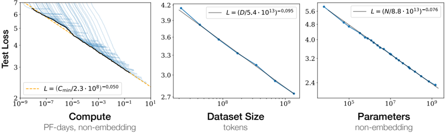
## Scaling Laws for Neural Language Models: Three-Plot Analysis ### Overview The image displays three horizontally arranged log-log plots, each illustrating a power-law relationship between a different scaling factor (Compute, Dataset Size, Parameters) and the Test Loss of a neural language model. The plots collectively demonstrate the "scaling laws" phenomenon, where model performance improves predictably as resources increase. ### Components/Axes The image is segmented into three distinct chart regions, each with its own axes and legend. **1. Left Chart: Compute vs. Test Loss** * **X-Axis:** `Compute` (Label: "Compute", Sub-label: "PF-days, non-embedding"). Scale is logarithmic, ranging from `10^-9` to `10^1`. * **Y-Axis:** `Test Loss` (Label: "Test Loss"). Scale is linear, ranging from `2` to `7`. * **Legend:** Located in the bottom-left corner. Contains a dashed orange line and the equation: `L = (C_min / 2.3 * 10^8)^-0.050`. * **Data Series:** A dense cloud of light blue data points, a solid black trend line passing through them, and a dashed orange extrapolation line extending the trend. **2. Middle Chart: Dataset Size vs. Test Loss** * **X-Axis:** `Dataset Size` (Label: "Dataset Size", Sub-label: "tokens"). Scale is logarithmic, ranging from `10^8` to `10^9`. * **Y-Axis:** `Test Loss` (Label: "Test Loss"). Scale is linear, ranging from `2.7` to `4.2`. * **Legend:** Located in the top-right corner. Contains a solid blue line and the equation: `L = (D / 5.4 * 10^13)^-0.095`. * **Data Series:** A series of blue data points connected by a solid blue trend line. **3. Right Chart: Parameters vs. Test Loss** * **X-Axis:** `Parameters` (Label: "Parameters", Sub-label: "non-embedding"). Scale is logarithmic, ranging from `10^5` to `10^9`. * **Y-Axis:** `Test Loss` (Label: "Test Loss"). Scale is linear, ranging from `2.4` to `5.6`. * **Legend:** Located in the top-right corner. Contains a solid blue line and the equation: `L = (N / 8.8 * 10^13)^-0.076`. * **Data Series:** A series of blue data points connected by a solid blue trend line. ### Detailed Analysis **Left Chart (Compute):** * **Trend Verification:** The data shows a clear downward trend. As Compute increases (moving right on the x-axis), Test Loss decreases (moving down on the y-axis). The relationship appears linear on this log-log plot, indicating a power law. * **Data Points & Equation:** The fitted power-law equation is `L ∝ C^-0.050`. The constant `C_min` is `2.3 * 10^8` PF-days. The exponent `-0.050` is the smallest in magnitude among the three plots, suggesting Test Loss decreases most slowly with increasing Compute. * **Spatial Grounding:** The dense cluster of light blue points is concentrated in the mid-to-high compute range (`10^-5` to `10^0`). The black trend line fits these points. The orange dashed line extrapolates the trend to lower and higher compute values. **Middle Chart (Dataset Size):** * **Trend Verification:** A strong, consistent downward trend. As Dataset Size increases, Test Loss decreases linearly on the log-log scale. * **Data Points & Equation:** The fitted power-law equation is `L ∝ D^-0.095`. The constant `D` is `5.4 * 10^13` tokens. The exponent `-0.095` is larger in magnitude than the compute exponent, indicating a steeper improvement in loss per decade of dataset growth. * **Spatial Grounding:** The blue data points are evenly spaced along the trend line from approximately `2*10^8` to `10^9` tokens. **Right Chart (Parameters):** * **Trend Verification:** A strong, consistent downward trend. As the number of Parameters increases, Test Loss decreases linearly on the log-log scale. * **Data Points & Equation:** The fitted power-law equation is `L ∝ N^-0.076`. The constant `N` is `8.8 * 10^13` parameters. The exponent `-0.076` is intermediate between the compute and dataset size exponents. * **Spatial Grounding:** The blue data points are evenly spaced along the trend line from approximately `10^6` to `10^9` parameters. ### Key Observations 1. **Universal Power-Law Scaling:** All three fundamental resources (Compute, Data, Parameters) exhibit a power-law relationship with model performance (Test Loss). This is a hallmark of neural scaling laws. 2. **Exponent Hierarchy:** The magnitude of the scaling exponent differs: Dataset Size (`-0.095`) > Parameters (`-0.076`) > Compute (`-0.050`). This suggests, within the observed ranges, that increasing the dataset size yields the most significant reduction in loss per unit of increase on a logarithmic scale. 3. **Smooth, Predictable Trends:** The data points align very closely with the fitted power-law lines, indicating highly predictable scaling behavior without significant outliers or plateaus in the observed regimes. 4. **Log-Log Linearity:** The linearity on log-log axes confirms the relationships are of the form `Loss ∝ (Resource)^-exponent`. ### Interpretation This image presents empirical evidence for the **scaling laws of neural language models**. The data demonstrates that model performance, measured by test loss, improves in a predictable, power-law fashion as three key resources are scaled up. * **What it Suggests:** The findings imply that performance gains are not arbitrary but follow a quantifiable trajectory. Researchers can use these fitted equations to forecast the expected loss for a given budget of compute, data, or parameters, enabling more efficient resource allocation for training large models. * **Relationship Between Elements:** The three plots are interconnected facets of the same phenomenon. In practice, scaling one resource (e.g., parameters) often requires scaling the others (compute for training, data for effective learning). The different exponents hint at the relative "efficiency" of each resource in reducing loss within the studied scale. * **Notable Implications:** The smooth, unbroken trends suggest that, up to the scales tested (e.g., ~1 trillion parameters, ~100 billion tokens), there is no fundamental "wall" or diminishing return that halts progress. This underpins the rationale behind the trend of building ever-larger models. The specific exponent values are critical for theoretical models that seek to explain why neural networks generalize and how to optimize the training triad of compute, data, and model size.

## Line Graphs: Test Loss vs Compute, Dataset Size, and Parameters ### Overview The image contains three line graphs comparing **Test Loss** against three variables: **Compute (PF-days, non-embedding)**, **Dataset Size (tokens)**, and **Parameters (non-embedding)**. Each graph includes a legend with mathematical equations describing the relationship between the variables and Test Loss. The graphs show downward trends, indicating that Test Loss decreases as the respective variables increase. --- ### Components/Axes #### Left Graph: Compute vs Test Loss - **X-axis**: Compute (PF-days, non-embedding) - Scale: Logarithmic (10⁻⁹ to 10¹) - **Y-axis**: Test Loss - Scale: Linear (2 to 7) - **Legend**: - Dashed orange line: `L = (C_min/2.3·10⁸)⁻⁰.⁰⁵⁰` - Multiple blue lines (density increases with Compute) #### Middle Graph: Dataset Size vs Test Loss - **X-axis**: Dataset Size (tokens) - Scale: Logarithmic (10⁸ to 10⁹) - **Y-axis**: Test Loss - Scale: Linear (2.7 to 4.2) - **Legend**: - Solid blue line: `L = (D/5.4·10¹³)⁻⁰.⁰⁹⁵` #### Right Graph: Parameters vs Test Loss - **X-axis**: Parameters (non-embedding) - Scale: Logarithmic (10⁵ to 10⁹) - **Y-axis**: Test Loss - Scale: Linear (2.4 to 5.6) - **Legend**: - Solid blue line: `L = (N/8.8·10¹³)⁻⁰.⁰⁷⁶` --- ### Detailed Analysis #### Left Graph: Compute vs Test Loss - **Trend**: Test Loss decreases as Compute increases. - **Data Points**: - Dashed orange line (theoretical model): - At 10⁻⁹ Compute: ~6.5 Test Loss - At 10¹ Compute: ~2.5 Test Loss - Blue lines (empirical data): - At 10⁻⁹ Compute: ~6.0–6.5 Test Loss - At 10¹ Compute: ~2.5–3.0 Test Loss - **Key Detail**: The orange line aligns closely with the densest cluster of blue lines, suggesting the equation approximates the trend. #### Middle Graph: Dataset Size vs Test Loss - **Trend**: Test Loss decreases as Dataset Size increases. - **Data Points**: - Solid blue line (theoretical model): - At 10⁸ tokens: ~3.9 Test Loss - At 10⁹ tokens: ~2.7 Test Loss - Empirical data points: - At 10⁸ tokens: ~3.6–3.9 Test Loss - At 10⁹ tokens: ~2.7–3.0 Test Loss - **Key Detail**: The solid line fits the data points tightly, confirming the equation’s accuracy. #### Right Graph: Parameters vs Test Loss - **Trend**: Test Loss decreases as Parameters increase. - **Data Points**: - Solid blue line (theoretical model): - At 10⁵ parameters: ~5.6 Test Loss - At 10⁹ parameters: ~2.4 Test Loss - Empirical data points: - At 10⁵ parameters: ~5.0–5.6 Test Loss - At 10⁹ parameters: ~2.4–2.8 Test Loss - **Key Detail**: The solid line closely matches the data, validating the equation. --- ### Key Observations 1. **Consistent Trends**: All three graphs show a clear inverse relationship between Test Loss and their respective variables. 2. **Theoretical vs. Empirical**: - The dashed orange line (left graph) and solid blue lines (middle/right graphs) align with empirical data, suggesting the equations model real-world behavior. 3. **Variability**: The left graph’s blue lines show greater spread at lower Compute values, possibly due to experimental noise or smaller sample sizes. --- ### Interpretation The data demonstrates that **Test Loss improves predictably** with increases in Compute, Dataset Size, or Parameters, following power-law relationships. The equations in the legends likely represent **scaling laws** common in machine learning, where performance gains diminish at higher resource levels. - **Compute**: The left graph’s orange line (`L = (C_min/2.3·10⁸)⁻⁰.⁰⁵⁰`) suggests Test Loss scales with the inverse square root of Compute. - **Dataset Size**: The middle graph’s blue line (`L = (D/5.4·10¹³)⁻⁰.⁰⁹⁵`) indicates Test Loss scales with the inverse 0.95th root of Dataset Size. - **Parameters**: The right graph’s blue line (`L = (N/8.8·10¹³)⁻⁰.⁰⁷⁶`) shows Test Loss scales with the inverse 0.76th root of Parameters. These relationships imply that optimizing these variables can systematically reduce Test Loss, though diminishing returns may occur at extreme scales (e.g., very high Compute or Parameters). The variability in the left graph highlights the importance of experimental consistency in low-resource regimes.