## Line Graphs: Test Loss vs Compute, Dataset Size, and Parameters
### Overview
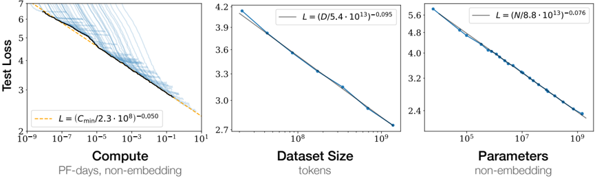
The image contains three line graphs comparing **Test Loss** against three variables: **Compute (PF-days, non-embedding)**, **Dataset Size (tokens)**, and **Parameters (non-embedding)**. Each graph includes a legend with mathematical equations describing the relationship between the variables and Test Loss. The graphs show downward trends, indicating that Test Loss decreases as the respective variables increase.
---
### Components/Axes
#### Left Graph: Compute vs Test Loss
- **X-axis**: Compute (PF-days, non-embedding)
- Scale: Logarithmic (10⁻⁹ to 10¹)
- **Y-axis**: Test Loss
- Scale: Linear (2 to 7)
- **Legend**:
- Dashed orange line: `L = (C_min/2.3·10⁸)⁻⁰.⁰⁵⁰`
- Multiple blue lines (density increases with Compute)
#### Middle Graph: Dataset Size vs Test Loss
- **X-axis**: Dataset Size (tokens)
- Scale: Logarithmic (10⁸ to 10⁹)
- **Y-axis**: Test Loss
- Scale: Linear (2.7 to 4.2)
- **Legend**:
- Solid blue line: `L = (D/5.4·10¹³)⁻⁰.⁰⁹⁵`
#### Right Graph: Parameters vs Test Loss
- **X-axis**: Parameters (non-embedding)
- Scale: Logarithmic (10⁵ to 10⁹)
- **Y-axis**: Test Loss
- Scale: Linear (2.4 to 5.6)
- **Legend**:
- Solid blue line: `L = (N/8.8·10¹³)⁻⁰.⁰⁷⁶`
---
### Detailed Analysis
#### Left Graph: Compute vs Test Loss
- **Trend**: Test Loss decreases as Compute increases.
- **Data Points**:
- Dashed orange line (theoretical model):
- At 10⁻⁹ Compute: ~6.5 Test Loss
- At 10¹ Compute: ~2.5 Test Loss
- Blue lines (empirical data):
- At 10⁻⁹ Compute: ~6.0–6.5 Test Loss
- At 10¹ Compute: ~2.5–3.0 Test Loss
- **Key Detail**: The orange line aligns closely with the densest cluster of blue lines, suggesting the equation approximates the trend.
#### Middle Graph: Dataset Size vs Test Loss
- **Trend**: Test Loss decreases as Dataset Size increases.
- **Data Points**:
- Solid blue line (theoretical model):
- At 10⁸ tokens: ~3.9 Test Loss
- At 10⁹ tokens: ~2.7 Test Loss
- Empirical data points:
- At 10⁸ tokens: ~3.6–3.9 Test Loss
- At 10⁹ tokens: ~2.7–3.0 Test Loss
- **Key Detail**: The solid line fits the data points tightly, confirming the equation’s accuracy.
#### Right Graph: Parameters vs Test Loss
- **Trend**: Test Loss decreases as Parameters increase.
- **Data Points**:
- Solid blue line (theoretical model):
- At 10⁵ parameters: ~5.6 Test Loss
- At 10⁹ parameters: ~2.4 Test Loss
- Empirical data points:
- At 10⁵ parameters: ~5.0–5.6 Test Loss
- At 10⁹ parameters: ~2.4–2.8 Test Loss
- **Key Detail**: The solid line closely matches the data, validating the equation.
---
### Key Observations
1. **Consistent Trends**: All three graphs show a clear inverse relationship between Test Loss and their respective variables.
2. **Theoretical vs. Empirical**:
- The dashed orange line (left graph) and solid blue lines (middle/right graphs) align with empirical data, suggesting the equations model real-world behavior.
3. **Variability**: The left graph’s blue lines show greater spread at lower Compute values, possibly due to experimental noise or smaller sample sizes.
---
### Interpretation
The data demonstrates that **Test Loss improves predictably** with increases in Compute, Dataset Size, or Parameters, following power-law relationships. The equations in the legends likely represent **scaling laws** common in machine learning, where performance gains diminish at higher resource levels.
- **Compute**: The left graph’s orange line (`L = (C_min/2.3·10⁸)⁻⁰.⁰⁵⁰`) suggests Test Loss scales with the inverse square root of Compute.
- **Dataset Size**: The middle graph’s blue line (`L = (D/5.4·10¹³)⁻⁰.⁰⁹⁵`) indicates Test Loss scales with the inverse 0.95th root of Dataset Size.
- **Parameters**: The right graph’s blue line (`L = (N/8.8·10¹³)⁻⁰.⁰⁷⁶`) shows Test Loss scales with the inverse 0.76th root of Parameters.
These relationships imply that optimizing these variables can systematically reduce Test Loss, though diminishing returns may occur at extreme scales (e.g., very high Compute or Parameters). The variability in the left graph highlights the importance of experimental consistency in low-resource regimes.