\n
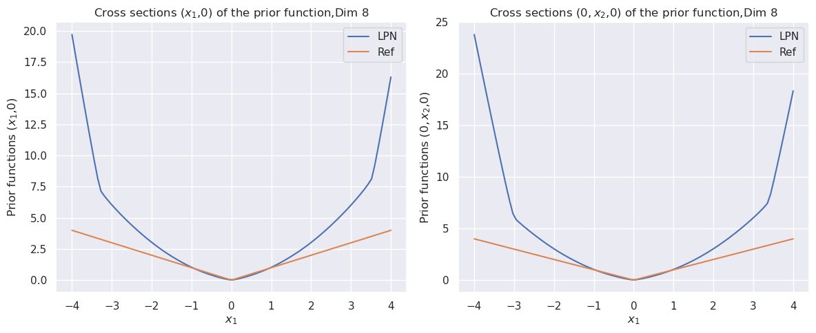
## [Line Charts]: Cross Sections of Prior Function (Dim 8)
### Overview
The image displays two side-by-side line charts comparing two functions, labeled "LPN" and "Ref," across different cross-sections of an 8-dimensional prior function. Both charts show the functions' behavior as a single variable changes while others are held at zero. The overall visual pattern is symmetric, with both functions reaching a minimum value of zero at the origin (x=0).
### Components/Axes
**Left Chart:**
* **Title:** `Cross sections (x₁,0) of the prior function,Dim 8`
* **Y-axis Label:** `Prior functions (x₁,0)`
* **X-axis Label:** `x₁`
* **Y-axis Scale:** Linear, ranging from 0.0 to 20.0, with major ticks at intervals of 2.5.
* **X-axis Scale:** Linear, ranging from -4 to 4, with major ticks at integer intervals.
* **Legend:** Located in the top-right corner. Contains two entries:
* `LPN` (blue line)
* `Ref` (orange line)
**Right Chart:**
* **Title:** `Cross sections (0, x₂,0) of the prior function,Dim 8`
* **Y-axis Label:** `Prior functions (0, x₂,0)`
* **X-axis Label:** `x₁` *(Note: This label appears inconsistent with the title, which references `x₂`. The axis variable is likely intended to be `x₂` based on the title.)*
* **Y-axis Scale:** Linear, ranging from 0 to 25, with major ticks at intervals of 5.
* **X-axis Scale:** Linear, ranging from -4 to 4, with major ticks at integer intervals.
* **Legend:** Located in the top-right corner. Contains the same two entries as the left chart:
* `LPN` (blue line)
* `Ref` (orange line)
### Detailed Analysis
**Left Chart - Cross Section (x₁,0):**
* **LPN (Blue Line):** Exhibits a pronounced, symmetric U-shape.
* **Trend:** Starts very high at the left extreme, decreases rapidly to a minimum at the center, then increases rapidly to a high value at the right extreme.
* **Approximate Data Points:**
* At x₁ = -4: y ≈ 19.8
* At x₁ = -3: y ≈ 7.0
* At x₁ = -2: y ≈ 3.0
* At x₁ = -1: y ≈ 1.0
* At x₁ = 0: y = 0.0
* At x₁ = 1: y ≈ 1.0
* At x₁ = 2: y ≈ 3.0
* At x₁ = 3: y ≈ 7.0
* At x₁ = 4: y ≈ 16.5
* **Ref (Orange Line):** Exhibits a symmetric V-shape, appearing linear on each side of the origin.
* **Trend:** Decreases linearly from the left to the origin, then increases linearly from the origin to the right.
* **Approximate Data Points:**
* At x₁ = -4: y ≈ 4.0
* At x₁ = 0: y = 0.0
* At x₁ = 4: y ≈ 4.0
**Right Chart - Cross Section (0, x₂,0):**
* **LPN (Blue Line):** Exhibits a symmetric U-shape, similar to the left chart but with a steeper ascent.
* **Trend:** Starts very high at the left extreme, decreases rapidly to a minimum at the center, then increases rapidly to a high value at the right extreme.
* **Approximate Data Points:**
* At x₁ (likely x₂) = -4: y ≈ 24.0
* At x₁ = -3: y ≈ 6.0
* At x₁ = -2: y ≈ 3.0
* At x₁ = -1: y ≈ 1.0
* At x₁ = 0: y = 0.0
* At x₁ = 1: y ≈ 1.0
* At x₁ = 2: y ≈ 3.0
* At x₁ = 3: y ≈ 7.0
* At x₁ = 4: y ≈ 18.5
* **Ref (Orange Line):** Exhibits a symmetric V-shape, identical in form to the left chart.
* **Trend:** Decreases linearly from the left to the origin, then increases linearly from the origin to the right.
* **Approximate Data Points:**
* At x₁ (likely x₂) = -4: y ≈ 4.0
* At x₁ = 0: y = 0.0
* At x₁ = 4: y ≈ 4.0
### Key Observations
1. **Symmetry:** Both functions (LPN and Ref) are perfectly symmetric around x=0 in both cross-sections.
2. **Minimum Point:** Both functions achieve their global minimum value of 0 at the origin (x=0).
3. **Relative Magnitude:** The LPN function has significantly higher values than the Ref function at all points except the origin. The disparity is greatest at the extremes (x=±4).
4. **Shape Difference:** The LPN function is a smooth, convex U-shape (suggesting a quadratic or higher-order polynomial relationship), while the Ref function is a piecewise-linear V-shape (suggesting an absolute value relationship).
5. **Cross-Section Comparison:** The LPN curve in the right chart (cross-section (0, x₂,0)) reaches a higher peak value (~24) at x=-4 compared to the left chart (~19.8), indicating the prior function may have different scaling or sensitivity along different dimensions.
6. **Label Discrepancy:** The x-axis on the right chart is labeled `x₁`, but the chart title references `x₂`. This is likely a labeling error, and the axis should represent `x₂`.
### Interpretation
The charts compare the behavior of a learned or proposed prior distribution ("LPN") against a reference prior ("Ref") in an 8-dimensional space. The data suggests the following:
* **Penalty for Deviation:** Both priors assign the lowest probability density (or highest "cost") to the origin (x=0) and increase as variables move away from zero. This is characteristic of priors that encourage sparsity or shrinkage towards zero.
* **LPN is More "Peaked":** The LPN prior penalizes deviations from zero much more severely than the Ref prior, especially for larger deviations. Its U-shape implies a stronger, non-linear push towards zero. This could indicate a more informative or restrictive prior designed to aggressively suppress non-zero values.
* **Reference Prior is Linear:** The Ref prior's V-shape corresponds to an L1-norm or Laplace prior, which applies a constant penalty per unit of deviation. This is a common choice for promoting sparsity.
* **Dimensional Anisotropy:** The difference in the LPN curve's height between the two cross-sections suggests the learned prior is not isotropic; its strength or shape varies depending on which dimension is being varied. This could be an intentional feature to model different importance of dimensions or an artifact of the learning process.
* **Purpose:** This visualization is likely used to validate or analyze the properties of a learned prior (LPN) by contrasting it with a standard, well-understood reference (Ref). It demonstrates that the LPN has successfully learned a prior that is qualitatively similar (symmetric, centered at zero) but quantitatively more aggressive in its shrinkage behavior.