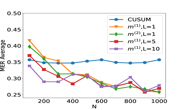
\n ## Line Chart: Performance Comparison of CUSUM and Modified Methods (MER Average vs. N) ### Overview The image is a line chart comparing the performance of five different statistical or algorithmic methods. The performance metric is "MER Average" (likely Mean Error Rate or a similar average error metric), plotted against a variable "N" (likely sample size, number of observations, or time steps). The chart shows how the average error changes for each method as N increases from approximately 100 to 1000. ### Components/Axes * **Chart Type:** Multi-line chart with markers. * **X-Axis:** * **Label:** `N` * **Scale:** Linear scale. * **Markers/Ticks:** Major ticks are labeled at 200, 400, 600, 800, and 1000. The axis starts slightly before 100 and ends at 1000. * **Y-Axis:** * **Label:** `MER Average` * **Scale:** Linear scale. * **Range:** 0.25 to 0.50. * **Markers/Ticks:** Major ticks are labeled at 0.25, 0.30, 0.35, 0.40, 0.45, and 0.50. * **Legend:** * **Position:** Top-right corner of the plot area. * **Entries (with color and marker):** 1. `CUSUM` - Blue line with circle markers. 2. `m^{(1)}, L=1` - Orange line with downward-pointing triangle markers. 3. `m^{(2)}, L=1` - Green line with diamond markers. 4. `m^{(1)}, L=5` - Red line with square markers. 5. `m^{(1)}, L=10` - Purple line with 'X' (cross) markers. ### Detailed Analysis **Trend Verification & Data Point Extraction (Approximate Values):** 1. **CUSUM (Blue, Circles):** * **Trend:** Relatively flat and stable across all N values, showing only minor fluctuations. It does not exhibit a strong downward or upward slope. * **Approximate Data Points:** * N≈100: ~0.36 * N≈200: ~0.35 * N≈300: ~0.35 * N≈400: ~0.35 * N≈500: ~0.355 * N≈600: ~0.36 * N≈700: ~0.35 * N≈800: ~0.35 * N≈900: ~0.35 * N≈1000: ~0.36 2. **m^{(1)}, L=1 (Orange, Downward Triangles):** * **Trend:** Shows a strong, consistent downward trend as N increases. It starts as the highest error method at low N and converges with the others at high N. * **Approximate Data Points:** * N≈100: ~0.42 (Highest initial point) * N≈200: ~0.365 * N≈300: ~0.355 * N≈400: ~0.315 * N≈500: ~0.31 * N≈600: ~0.29 * N≈700: ~0.275 * N≈800: ~0.275 * N≈900: ~0.26 * N≈1000: ~0.265 3. **m^{(2)}, L=1 (Green, Diamonds):** * **Trend:** Also shows a strong downward trend, very similar in shape to the orange line (m^{(1)}, L=1), but consistently slightly lower in error for most N values. * **Approximate Data Points:** * N≈100: ~0.40 * N≈200: ~0.36 * N≈300: ~0.315 * N≈400: ~0.315 * N≈500: ~0.305 * N≈600: ~0.285 * N≈700: ~0.27 * N≈800: ~0.275 * N≈900: ~0.265 * N≈1000: ~0.26 4. **m^{(1)}, L=5 (Red, Squares):** * **Trend:** General downward trend, but with more volatility (ups and downs) compared to the L=1 variants. It starts lower than the L=1 methods at N=100. * **Approximate Data Points:** * N≈100: ~0.37 * N≈200: ~0.33 * N≈300: ~0.31 * N≈400: ~0.285 * N≈500: ~0.305 * N≈600: ~0.28 * N≈700: ~0.28 * N≈800: ~0.29 * N≈900: ~0.26 * N≈1000: ~0.27 5. **m^{(1)}, L=10 (Purple, Crosses):** * **Trend:** Shows the most volatile behavior. It starts with the lowest error at N=100, drops sharply, then fluctuates significantly, rising notably at N=400 and N=800 before dropping again. * **Approximate Data Points:** * N≈100: ~0.34 (Lowest initial point) * N≈200: ~0.29 * N≈300: ~0.29 * N≈400: ~0.315 * N≈500: ~0.31 * N≈600: ~0.275 * N≈700: ~0.275 * N≈800: ~0.305 * N≈900: ~0.265 * N≈1000: ~0.28 ### Key Observations 1. **Convergence:** All four `m` methods (orange, green, red, purple) show a general trend of decreasing MER Average as N increases, converging into a narrow band between approximately 0.26 and 0.28 by N=1000. 2. **CUSUM Stability:** The CUSUM method (blue) is distinct, maintaining a nearly constant error rate (~0.35-0.36) regardless of N, making it the worst-performing method for N > 300. 3. **Impact of L:** For the `m^{(1)}` family, increasing the parameter `L` from 1 to 5 to 10 changes the behavior: * `L=1` (orange): Smooth, steady decline. * `L=5` (red): More volatile decline. * `L=10` (purple): Highly volatile, with significant local maxima at N=400 and N=800. 4. **Initial Performance:** At the smallest N (~100), the methods rank from highest to lowest error: `m^{(1)}, L=1` > `m^{(2)}, L=1` > `m^{(1)}, L=5` > `CUSUM` > `m^{(1)}, L=10`. 5. **Final Performance:** At the largest N (1000), the `m` methods are tightly clustered, while CUSUM remains an outlier with significantly higher error. ### Interpretation This chart likely evaluates change-point detection or sequential analysis algorithms. "MER Average" probably stands for Mean Detection Error Rate or a similar metric combining false alarms and missed detections. "N" represents the amount of data processed. The data suggests that the proposed `m` methods (variants with parameters `m` and `L`) are **adaptive and improve with more data**, learning to reduce their error rate as N grows. In contrast, the standard CUSUM algorithm appears **non-adaptive** in this context, with a fixed performance profile that does not benefit from increased sample size within this range. The parameter `L` seems to control a **memory or window length**. A smaller `L` (L=1) leads to stable, predictable improvement. A larger `L` (L=10) introduces volatility, suggesting the algorithm might be overfitting to local patterns or experiencing delayed reactions, causing temporary performance degradation (the peaks at N=400 and 800) before correcting. The `m^{(2)}` variant (green) performs very similarly to `m^{(1)}, L=1` (orange), indicating that the change from `m^{(1)}` to `m^{(2)}` has a minor effect compared to changing `L`. **In essence:** For large datasets (high N), the adaptive `m` methods are superior to CUSUM. If stability is crucial, a lower `L` value is preferable. If the lowest possible error at very small N is the goal, a high `L` value (`L=10`) might be chosen, accepting its subsequent volatility.