## Scatter Plot: Average Test-Time Compute by Game Configuration for Two Models
### Overview
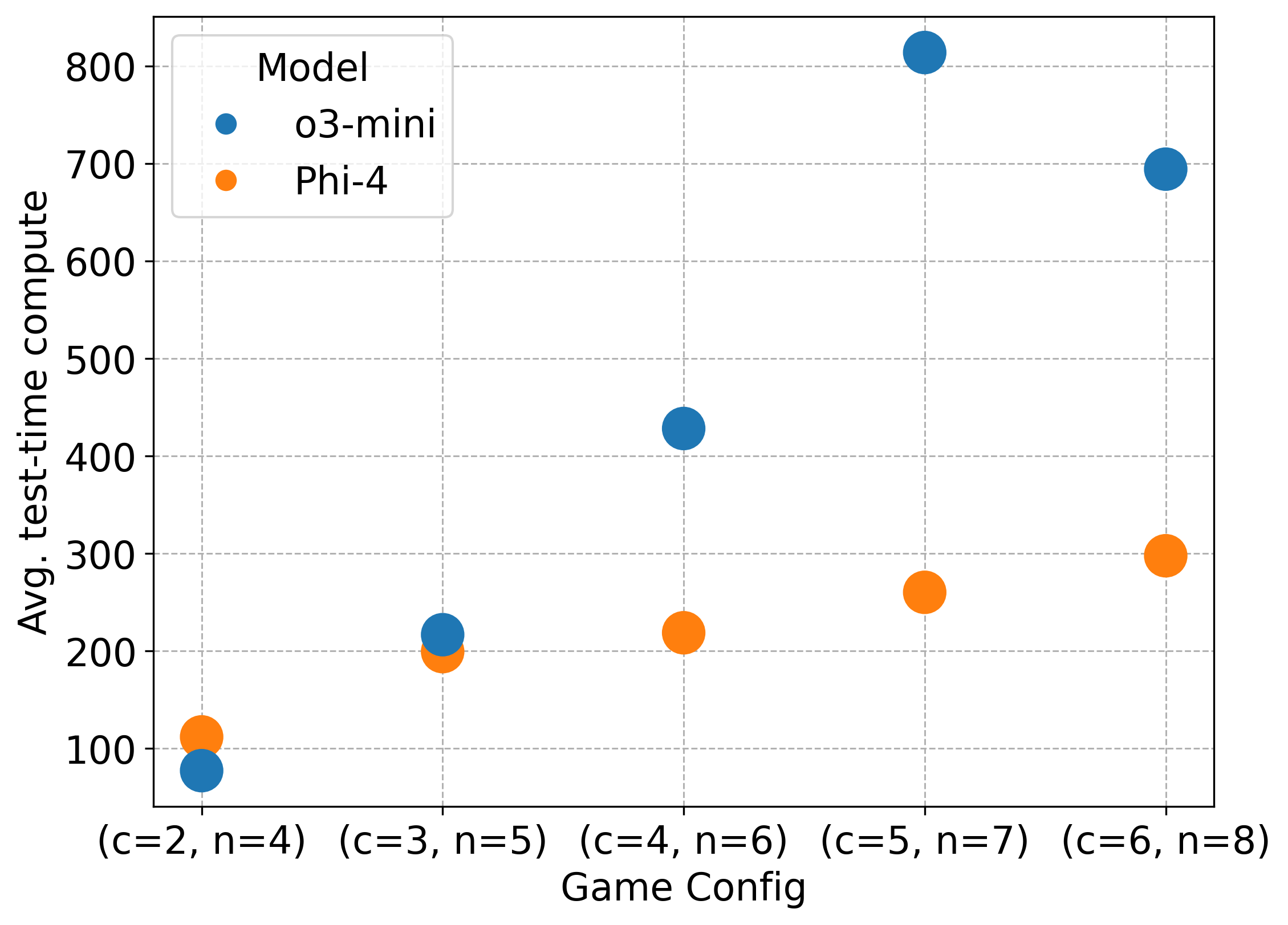
The image is a scatter plot comparing the average test-time compute (y-axis) of two AI models, "o3-mini" and "Phi-4", across five different game configurations (x-axis). The plot uses colored circles to represent data points for each model at each configuration.
### Components/Axes
* **Chart Type:** Scatter Plot
* **X-Axis:**
* **Title:** "Game Config"
* **Categories/Labels (from left to right):**
1. `(c=2, n=4)`
2. `(c=3, n=5)`
3. `(c=4, n=6)`
4. `(c=5, n=7)`
5. `(c=6, n=8)`
* **Y-Axis:**
* **Title:** "Avg. test-time compute"
* **Scale:** Linear, ranging from approximately 50 to 850.
* **Major Tick Marks:** 100, 200, 300, 400, 500, 600, 700, 800.
* **Legend:**
* **Position:** Top-left corner of the plot area.
* **Title:** "Model"
* **Series:**
* Blue circle: `o3-mini`
* Orange circle: `Phi-4`
### Detailed Analysis
Data points are extracted by matching the color of the circle to the legend and reading its approximate position against the y-axis grid.
**1. Game Config: (c=2, n=4)**
* **o3-mini (Blue):** Positioned just below the 100 line. Approximate value: **~80**.
* **Phi-4 (Orange):** Positioned just above the 100 line. Approximate value: **~110**.
**2. Game Config: (c=3, n=5)**
* **o3-mini (Blue):** Positioned slightly above the 200 line. Approximate value: **~220**.
* **Phi-4 (Orange):** Positioned just below the 200 line. Approximate value: **~195**.
**3. Game Config: (c=4, n=6)**
* **o3-mini (Blue):** Positioned between the 400 and 500 lines, closer to 400. Approximate value: **~430**.
* **Phi-4 (Orange):** Positioned just above the 200 line. Approximate value: **~220**.
**4. Game Config: (c=5, n=7)**
* **o3-mini (Blue):** Positioned just above the 800 line. Approximate value: **~820**.
* **Phi-4 (Orange):** Positioned between the 200 and 300 lines, closer to 300. Approximate value: **~260**.
**5. Game Config: (c=6, n=8)**
* **o3-mini (Blue):** Positioned on the 700 line. Approximate value: **~700**.
* **Phi-4 (Orange):** Positioned on the 300 line. Approximate value: **~300**.
### Key Observations
* **Diverging Trends:** The two models exhibit fundamentally different scaling behaviors.
* **o3-mini (Blue):** Shows a steep, non-linear increase in compute from config 1 to 4, peaking at config 4 (`c=5, n=7`), followed by a significant drop at config 5 (`c=6, n=8`). The trend is sharply upward then downward.
* **Phi-4 (Orange):** Shows a steady, near-linear increase in compute across all five configurations. The trend is consistently upward.
* **Crossover Point:** At the simplest configuration (`c=2, n=4`), Phi-4 uses slightly more compute than o3-mini. By the second configuration (`c=3, n=5`), o3-mini's compute surpasses Phi-4's, and the gap widens dramatically thereafter.
* **Peak Compute:** The highest compute value on the chart is for o3-mini at configuration `(c=5, n=7)` (~820). The lowest is for o3-mini at `(c=2, n=4)` (~80).
* **Anomaly:** The data point for o3-mini at `(c=6, n=8)` (~700) is a notable drop from its peak at the previous configuration, breaking its prior steep upward trend.
### Interpretation
This chart visualizes the computational cost (test-time compute) of running two different AI models on tasks of increasing complexity, parameterized by `c` and `n` (likely representing game or problem dimensions).
The data suggests a critical trade-off in model architecture or strategy:
* **Phi-4** demonstrates **predictable, scalable efficiency**. Its compute requirements grow proportionally and manageably with problem size, making it potentially more suitable for scaling to very complex tasks where resource predictability is key.
* **o3-mini** exhibits **highly variable, non-linear scaling**. It is very efficient for simple tasks but its computational cost explodes for mid-range complexity before dropping for the most complex task shown. This could indicate an internal strategy shift, a different algorithmic approach that becomes inefficient at certain scales, or that the model hits a performance ceiling and changes its behavior. The drop at the final data point is particularly intriguing—it may suggest the model fails or adopts a much simpler (and cheaper) strategy for the most complex configuration.
In essence, the chart doesn't just show "which model is faster," but reveals **how their underlying computational strategies respond to scaling pressure**. Phi-4 appears robust and consistent, while o3-mini's performance is highly sensitive to the specific problem parameters, with a potential breakdown or phase change at high complexity.