## Log-Log Plot: Trailing LM Loss vs. Computational Cost (PFLOP/s-days)
### Overview
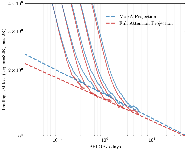
The image is a technical log-log plot comparing the performance scaling of two different projection methods for language models. It plots the "Trailing LM loss" against the computational cost measured in "PFLOP/s-days". The chart demonstrates how model loss decreases as computational resources increase for both methods, with one method consistently outperforming the other.
### Components/Axes
* **Chart Type:** Log-Log Line Plot.
* **Y-Axis (Vertical):**
* **Label:** `Trailing LM loss (seqlen=32K, last 2K)`
* **Scale:** Logarithmic (base 10).
* **Major Tick Marks:** `10^0` (1), `2×10^0` (2), `3×10^0` (3), `4×10^0` (4).
* **Interpretation:** This measures the language model's loss (lower is better) on the final 2,000 tokens of a 32,000-token sequence.
* **X-Axis (Horizontal):**
* **Label:** `PFLOP/s-days`
* **Scale:** Logarithmic (base 10).
* **Major Tick Marks:** `10^-1` (0.1), `10^0` (1), `10^1` (10).
* **Interpretation:** This is a unit of computational cost, representing Peta (10^15) Floating-Point Operations per second sustained over a number of days.
* **Legend:**
* **Position:** Top-right corner of the plot area.
* **Entry 1:** `MoBA Projection` - Represented by a blue, dashed line (`--`).
* **Entry 2:** `Full Attention Projection` - Represented by a red, dashed line (`--`).
* **Data Series:** The plot contains multiple lines for each projection type. There are approximately 5-6 distinct blue dashed lines (MoBA) and 5-6 distinct red dashed lines (Full Attention). Each pair of a blue and red line likely corresponds to a specific model configuration or size, though these are not individually labeled in the image.
### Detailed Analysis
* **General Trend:** All lines on the plot slope downwards from left to right. This indicates a clear inverse relationship: as computational cost (PFLOP/s-days) increases, the trailing LM loss decreases. The relationship appears linear on this log-log scale, suggesting a power-law relationship between loss and compute.
* **Method Comparison:** For any given x-value (computational cost), the red dashed lines (`Full Attention Projection`) are consistently positioned **below** the corresponding blue dashed lines (`MoBA Projection`). This visual relationship holds true across the entire range of the x-axis shown (from ~0.05 to ~30 PFLOP/s-days).
* **Line Groupings:** The lines are not evenly spaced. They appear in clustered pairs (one blue, one red). The vertical gap between a blue line and its paired red line appears relatively consistent across the x-axis for each pair. The pairs themselves are spread vertically, with some starting at higher loss values (top of the chart) and others starting lower.
* **Specific Value Points (Approximate):**
* At `10^0` (1) PFLOP/s-day:
* The lowest red line is at approximately `1.3` loss.
* The corresponding lowest blue line is at approximately `1.5` loss.
* The highest visible red line is near `4.0` loss.
* The corresponding highest visible blue line is above `4.0` loss (off the top of the chart).
* At `10^1` (10) PFLOP/s-days:
* The lowest red line approaches `1.0` loss.
* The corresponding lowest blue line is slightly above `1.0` loss.
* The lines converge toward the bottom-right corner of the plot.
### Key Observations
1. **Consistent Performance Gap:** The `Full Attention Projection` method demonstrates a consistent and significant advantage over the `MoBA Projection` method. For the same computational budget, it achieves a lower language model loss.
2. **Power-Law Scaling:** The linear trend on the log-log plot for all series confirms that loss scales as a power law with increased compute (`Loss ∝ Compute^(-α)`), a common finding in neural scaling laws.
3. **Parallel Trajectories:** The paired lines for each model configuration appear roughly parallel, suggesting that the scaling exponent (the slope, `α`) is similar between the two projection methods for a given model, but the constant factor (the vertical offset) favors Full Attention.
4. **Convergence at High Compute:** The lines appear to converge as they approach the bottom-right of the chart (high compute, low loss), suggesting the performance gap may narrow at extremely large scales, though it remains present within the plotted range.
### Interpretation
This chart provides empirical evidence for a comparative analysis of two architectural choices in language modeling: **MoBA (Mixture of Block Attention) Projection** versus **Full Attention Projection**.
* **What the data suggests:** The data strongly suggests that, under the measured conditions (seqlen=32K, evaluating on the last 2K tokens), the Full Attention mechanism is more **compute-efficient** than the MoBA Projection. It achieves a better (lower) loss for an identical amount of computational resources spent.
* **Relationship between elements:** The x-axis (compute) is the independent variable, and the y-axis (loss) is the dependent variable. The different line pairs represent different model scales or configurations. The key relationship highlighted is the **efficiency frontier**: the Full Attention lines define a better frontier (lower loss for given compute) than the MoBA lines.
* **Notable implications:** The consistent gap implies that the potential efficiency gains promised by sparse attention methods like MoBA may not fully materialize in this specific evaluation metric and setup, or that they come at a cost to model quality (higher loss). The power-law scaling confirms both methods are viable and improve predictably with scale, but Full Attention maintains a constant-factor advantage. This kind of analysis is critical for making informed architectural decisions when allocating massive computational budgets for training large language models. The "Trailing LM loss" metric specifically tests the model's ability to use long-context information effectively, suggesting Full Attention may be superior for this particular aspect of long-context reasoning.