## Contour Plot: State Space Convergence ### Overview The image is a contour plot showing the convergence of a system's state space over time. It displays a series of nested polygons, each representing the state space at a different time step. The outermost red rectangle, labeled "Ωε", defines the boundaries of the plot. The nested polygons converge towards the center, indicating the system's state is stabilizing. ### Components/Axes * **X-axis (x1):** Ranges from -0.03 to 0.03, with tick marks at -0.03, -0.02, -0.01, 0, 0.01, 0.02, and 0.03. * **Y-axis (x2):** Ranges from -0.01 to 0.07, with tick marks at -0.01, 0, 0.01, 0.02, 0.03, 0.04, 0.05, 0.06, and 0.07. * **Legend:** Located in the top-right corner, it identifies the red rectangle as "Ωε". * **Contours:** A series of nested polygons, each represented by a different color. These polygons represent the state space at different time steps. ### Detailed Analysis * **Outer Boundary (Ωε):** A red rectangle with corners at approximately (-0.025, -0.01), (0.03, -0.01), (0.03, 0.065), and (-0.025, 0.065). * **Convergence:** The nested polygons converge towards the center of the plot. The polygons are colored with a variety of colors, including light blue, green, yellow, orange, red, purple, and dark blue. * **Shape Change:** The shape of the polygons changes as they converge, becoming more compact and regular. The innermost polygon is roughly hexagonal. ### Key Observations * The system's state space shrinks over time, indicating stability. * The rate of convergence appears to decrease as the polygons get closer to the center. * The final state space is contained within a small region around the origin. ### Interpretation The contour plot illustrates the convergence of a dynamic system's state space. The nested polygons represent the reachable states of the system at different points in time. The fact that these polygons shrink and converge towards the center indicates that the system is stable and its state is approaching a steady-state value. The shape of the polygons provides information about the system's dynamics and how it evolves over time. The outer boundary, Ωε, likely represents a constraint or limit on the system's state space.

\n ## Contour Plot: State Space Representation ### Overview The image presents a contour plot visualizing a two-dimensional state space. The plot displays multiple closed curves, representing level sets of some function of two variables, x₁ and x₂. The plot is enclosed in a red rectangular border. A legend in the top-right corner identifies the curves as representing Ωε. ### Components/Axes * **X-axis:** Labeled "x₁", ranging from approximately -0.03 to 0.03. * **Y-axis:** Labeled "x₂", ranging from approximately -0.01 to 0.07. * **Contours:** Multiple closed curves representing different values of Ωε. * **Legend:** Located in the top-right corner, labeling the curves as "Ωε" and using a solid red line to represent them. * **Border:** A red rectangular border encompasses the entire plot. ### Detailed Analysis The contour plot shows a series of nested, elliptical-like contours. The contours are most densely packed near the origin (x₁ ≈ 0, x₂ ≈ 0), indicating a region of high concentration or a local maximum of the function represented by Ωε. As you move away from the origin, the contours become more spaced out, suggesting a decreasing value of Ωε. The contours exhibit an elongated shape, oriented diagonally. The highest concentration of contours appears to be centered around the point (x₁ ≈ 0, x₂ ≈ 0.03). The contours are generally smooth and continuous, with no apparent discontinuities or sharp corners. It's difficult to extract precise numerical values from the contours without knowing the specific function Ωε. However, we can observe the relative positions and densities of the contours to infer the behavior of the function. ### Key Observations * **Concentration:** The highest concentration of contours is near (0, 0.03). * **Elongation:** The contours are elongated diagonally. * **Density Gradient:** Contour density decreases as you move away from the origin. * **Shape:** The contours are generally elliptical. ### Interpretation This contour plot likely represents the state space of a dynamical system. The contours represent the level sets of a Lyapunov function (Ωε), which is used to analyze the stability of the system. The region enclosed by the innermost contours represents a stable region, where the system's trajectories will converge. The red border may indicate the boundaries of the state space or a region of interest. The elongated shape of the contours suggests that the system's dynamics are anisotropic, meaning that the system's behavior is different in different directions. The concentration of contours near the origin indicates that the system is most stable near that point. The plot suggests that the system has a stable equilibrium point near (0, 0.03). The shape and density of the contours provide information about the system's stability and the behavior of its trajectories. Without knowing the specific function Ωε, it is difficult to provide a more detailed interpretation. The plot is a visualization of a two-dimensional phase space, and the contours represent the paths of constant energy or some other conserved quantity. The red rectangle likely defines the region of interest or the boundaries of the system.

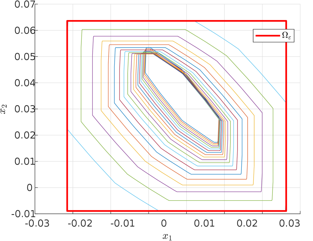
## Contour Plot / Phase Portrait: Nested Polygons within a Bounding Rectangle ### Overview The image is a 2D technical plot displaying a series of nested, closed polygons (likely representing contour lines or level sets) contained within a prominent red rectangular boundary. The plot is set against a light gray grid on a white background. The visualization appears to represent a mathematical or engineering concept, such as a stability region, invariant set, or phase portrait of a dynamical system. ### Components/Axes * **Plot Type:** 2D contour plot or phase portrait. * **Axes:** * **Horizontal Axis (x1):** Labeled `x1`. The scale runs from approximately -0.03 to 0.03. Major tick marks are present at intervals of 0.01 (e.g., -0.03, -0.02, -0.01, 0, 0.01, 0.02, 0.03). * **Vertical Axis (x2):** Labeled `x2`. The scale runs from approximately -0.01 to 0.07. Major tick marks are present at intervals of 0.01 (e.g., -0.01, 0, 0.01, 0.02, 0.03, 0.04, 0.05, 0.06, 0.07). * **Legend:** Located in the top-right corner of the plot area. It contains a single entry: a thick red line segment labeled with the mathematical symbol **Ωε** (Omega subscript epsilon). * **Primary Boundary:** A thick, solid red rectangle, corresponding to the legend entry **Ωε**. Its approximate corners are at coordinates (-0.022, -0.009) and (0.029, 0.064). * **Data Series (Nested Polygons):** A set of approximately 20-25 concentric, closed polygons. Each polygon is drawn with a thin line of a distinct color. The colors include (from outermost to innermost, approximate sequence): light blue, green, purple, yellow, orange, red, dark blue, and others, repeating in a pattern. The polygons are not perfect circles or ellipses but have a distinct, slightly irregular, multi-faceted shape, suggesting they are defined by a piecewise-linear or polyhedral function. ### Detailed Analysis * **Spatial Arrangement:** The polygons are nested concentrically. The outermost polygon is the largest, and each subsequent polygon is contained within the previous one, with the innermost polygon being the smallest. They are all centered roughly around the point (0.005, 0.035). * **Shape & Trend:** All polygons share a similar geometric characteristic: they are elongated along a diagonal axis running from the top-left to the bottom-right of the plot. The shapes are not symmetric about the x1 or x2 axes. The trend is a clear convergence towards a central point or region. * **Color-Legend Cross-Reference:** The red color is exclusively used for the outer bounding rectangle labeled **Ωε**. None of the inner nested polygons are red. The inner polygons use a palette of other colors (blues, greens, purples, yellows, oranges) which are not individually labeled in a legend. * **Data Point Approximation (Polygon Vertices):** While exact vertices are not labeled, the polygons' corners can be approximated relative to the grid. For example, the outermost light blue polygon has a vertex near (0.025, 0.030) and another near (-0.020, 0.022). The innermost polygons are tightly clustered around the central point. ### Key Observations 1. **Concentric Nesting:** The most striking feature is the perfect nesting of the polygons, indicating a hierarchical or iterative relationship between them. 2. **Diagonal Orientation:** The consistent diagonal elongation of all shapes suggests an underlying dynamic or constraint that is not aligned with the primary x1 or x2 axes. 3. **Bounding Set:** The red rectangle **Ωε** acts as a strict outer boundary. All other data (the polygons) are fully contained within it. 4. **Lack of Individual Labels:** The inner polygons are not individually identified. Their meaning is derived from their collective pattern and relationship to the bounding set **Ωε**. ### Interpretation This plot is highly characteristic of visualizations used in **control theory, optimization, or dynamical systems analysis**. * **What it likely represents:** The nested polygons are almost certainly **level sets** (contours) of a scalar function, such as a **Lyapunov function** or a **cost function**. The function's value decreases as one moves from the outer polygons toward the center. The central point (approx. 0.005, 0.035) is likely an **equilibrium point** or an **optimal solution**. * **Role of Ωε:** The red rectangle **Ωε** defines a **region of interest, a safe operating set, or an invariant set**. The fact that all level sets are contained within it suggests that trajectories starting inside **Ωε** will remain within it and converge toward the central equilibrium. The subscript ε (epsilon) often denotes a small, positive parameter, implying this set might be defined by a tolerance or a bound. * **Underlying System:** The diagonal, non-axis-aligned shape of the contours indicates that the system's dynamics or the function's Hessian have coupled terms between the states `x1` and `x2`. The system is not decoupled. * **Purpose:** The graph demonstrates **stability** or **convergence**. It visually proves that from any point within the bounding set **Ωε**, the system state will evolve (following the gradient of the function) toward the central equilibrium, as shown by the descending sequence of level sets. It is a graphical certificate of performance for a controller or an optimization algorithm.

## Contour Plot: Level Sets of Ωε(x₁, x₂) ### Overview The image depicts a contour plot of a two-dimensional function Ωε(x₁, x₂), represented by nested polygonal lines. The outermost contour is a red square labeled Ωε, while inner contours form increasingly complex polygons with varying numbers of sides. The plot spans x₁ ∈ [-0.03, 0.03] and x₂ ∈ [-0.01, 0.07], with contour lines denser near the origin (0,0). ### Components/Axes - **Axes**: - **x₁ (horizontal)**: Ranges from -0.03 to 0.03, labeled at intervals of 0.01. - **x₂ (vertical)**: Ranges from -0.01 to 0.07, labeled at intervals of 0.01. - **Legend**: Located in the top-right corner, explicitly labeling the red contour as Ωε. No other legend entries are visible. - **Contour Lines**: - **Ωε (red)**: Forms a square boundary at the plot's perimeter. - **Inner contours**: Progressively smaller polygons (octagons, decagons, etc.) with colors transitioning from purple to green to blue as they approach the center. ### Detailed Analysis 1. **Ωε Contour (Red)**: - Forms a perfect square with vertices at (±0.03, ±0.07). - Acts as the maximum boundary for Ωε. 2. **Inner Contours**: - **Color progression**: Purple → Orange → Red → Blue → Green (approximate, based on visual gradient). - **Shape evolution**: Square → Octagon → Decagon → Irregular polygons → Near-circular shapes near the origin. - **Spacing**: Contours are evenly spaced in the outer regions but become denser (closer together) as they approach the center, suggesting a steeper gradient of Ωε near (0,0). 3. **Symmetry**: - The plot exhibits approximate symmetry about both axes, though the x₂ range is asymmetric (positive bias). ### Key Observations - **Convergence to Origin**: All contours collapse to a single point at (0,0), indicating a critical point (likely a minimum or saddle point) for Ωε. - **Shape Transition**: The shift from regular polygons to irregular shapes near the center suggests a nonlinear relationship between Ωε and spatial coordinates. - **Asymmetry in x₂**: The upper x₂ limit (0.07) is twice the lower limit (-0.01), potentially reflecting boundary conditions or domain constraints. ### Interpretation The plot visualizes level sets of Ωε, where each contour represents a constant value of the function. The red Ωε contour defines the domain's outer boundary, while inner contours map regions of decreasing Ωε values. The convergence to a point at the origin implies a singularity or extremum there. The transition from square to rounded contours may indicate a change in the function's curvature or interaction with domain boundaries. The lack of labeled inner contours prevents quantitative analysis, but the spatial density suggests Ωε varies most rapidly near the origin. This structure is typical of potential fields, stress distributions, or optimization landscapes in technical applications.