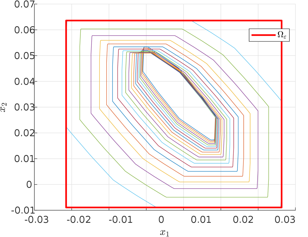
\n ## Contour Plot: State Space Representation ### Overview The image presents a contour plot visualizing a two-dimensional state space. The plot displays multiple closed curves, representing level sets of some function of two variables, x₁ and x₂. The plot is enclosed in a red rectangular border. A legend in the top-right corner identifies the curves as representing Ωε. ### Components/Axes * **X-axis:** Labeled "x₁", ranging from approximately -0.03 to 0.03. * **Y-axis:** Labeled "x₂", ranging from approximately -0.01 to 0.07. * **Contours:** Multiple closed curves representing different values of Ωε. * **Legend:** Located in the top-right corner, labeling the curves as "Ωε" and using a solid red line to represent them. * **Border:** A red rectangular border encompasses the entire plot. ### Detailed Analysis The contour plot shows a series of nested, elliptical-like contours. The contours are most densely packed near the origin (x₁ ≈ 0, x₂ ≈ 0), indicating a region of high concentration or a local maximum of the function represented by Ωε. As you move away from the origin, the contours become more spaced out, suggesting a decreasing value of Ωε. The contours exhibit an elongated shape, oriented diagonally. The highest concentration of contours appears to be centered around the point (x₁ ≈ 0, x₂ ≈ 0.03). The contours are generally smooth and continuous, with no apparent discontinuities or sharp corners. It's difficult to extract precise numerical values from the contours without knowing the specific function Ωε. However, we can observe the relative positions and densities of the contours to infer the behavior of the function. ### Key Observations * **Concentration:** The highest concentration of contours is near (0, 0.03). * **Elongation:** The contours are elongated diagonally. * **Density Gradient:** Contour density decreases as you move away from the origin. * **Shape:** The contours are generally elliptical. ### Interpretation This contour plot likely represents the state space of a dynamical system. The contours represent the level sets of a Lyapunov function (Ωε), which is used to analyze the stability of the system. The region enclosed by the innermost contours represents a stable region, where the system's trajectories will converge. The red border may indicate the boundaries of the state space or a region of interest. The elongated shape of the contours suggests that the system's dynamics are anisotropic, meaning that the system's behavior is different in different directions. The concentration of contours near the origin indicates that the system is most stable near that point. The plot suggests that the system has a stable equilibrium point near (0, 0.03). The shape and density of the contours provide information about the system's stability and the behavior of its trajectories. Without knowing the specific function Ωε, it is difficult to provide a more detailed interpretation. The plot is a visualization of a two-dimensional phase space, and the contours represent the paths of constant energy or some other conserved quantity. The red rectangle likely defines the region of interest or the boundaries of the system.