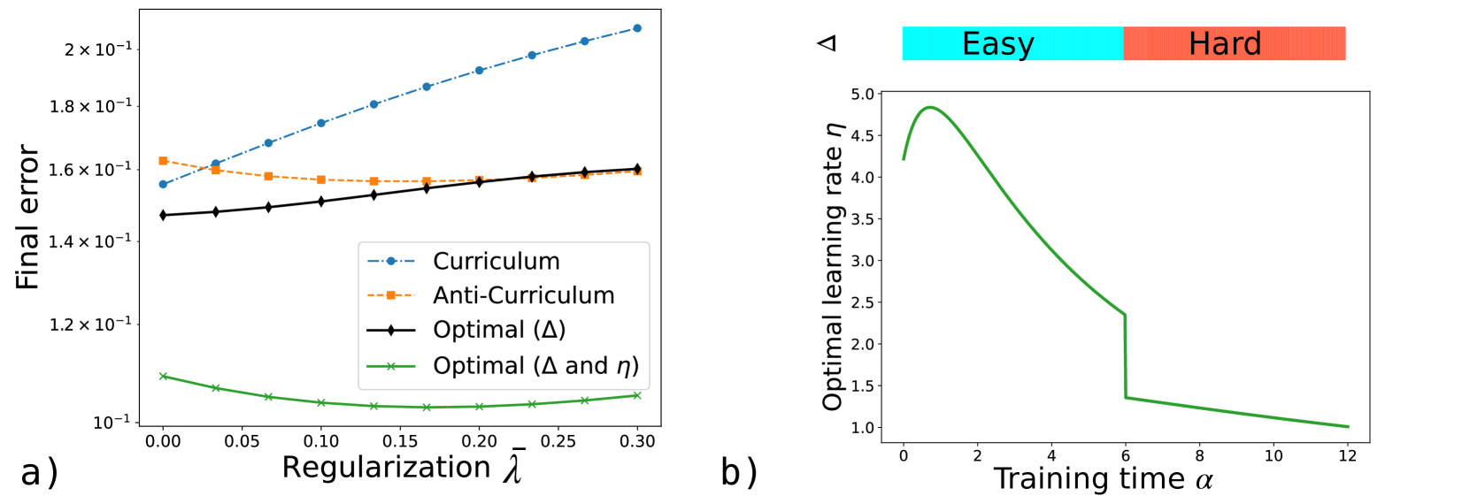
## Charts: Training Performance Analysis ### Overview The image presents two charts (a and b) analyzing the performance of different training strategies. Chart a) shows the final error as a function of regularization strength (λ) for Curriculum, Anti-Curriculum, Optimal (Δ), and Optimal (Δ and η) methods. Chart b) depicts the optimal learning rate (η) as a function of training time (α), segmented into "Easy" and "Hard" phases. ### Components/Axes **Chart a):** * **X-axis:** Regularization λ (ranging from approximately 0.00 to 0.30) * **Y-axis:** Final error (logarithmic scale, ranging from approximately 1.0 x 10⁻¹ to 2.0 x 10⁻¹) * **Data Series:** * Curriculum (blue dashed line with circle markers) * Anti-Curriculum (orange dashed line with triangle markers) * Optimal (Δ) (black solid line with circle markers) * Optimal (Δ and η) (green solid line with cross markers) * **Legend:** Located in the bottom-left corner, associating colors with each data series. **Chart b):** * **X-axis:** Training time α (ranging from approximately 0.00 to 12.0) * **Y-axis:** Optimal learning rate η (ranging from approximately 0.8 to 5.2) * **Segmentation:** The chart is visually divided into two regions: "Easy" (green background, α < ~6) and "Hard" (red background, α > ~6). * **Data Series:** A single green solid line representing the optimal learning rate. ### Detailed Analysis or Content Details **Chart a):** * **Curriculum:** The line slopes upward, indicating that as regularization strength increases, the final error also increases. * λ = 0.00: Error ≈ 1.55 x 10⁻¹ * λ = 0.05: Error ≈ 1.58 x 10⁻¹ * λ = 0.10: Error ≈ 1.65 x 10⁻¹ * λ = 0.15: Error ≈ 1.75 x 10⁻¹ * λ = 0.20: Error ≈ 1.85 x 10⁻¹ * λ = 0.25: Error ≈ 1.95 x 10⁻¹ * λ = 0.30: Error ≈ 2.05 x 10⁻¹ * **Anti-Curriculum:** The line initially decreases and then plateaus, suggesting a limited benefit from increased regularization. * λ = 0.00: Error ≈ 1.65 x 10⁻¹ * λ = 0.05: Error ≈ 1.60 x 10⁻¹ * λ = 0.10: Error ≈ 1.55 x 10⁻¹ * λ = 0.15: Error ≈ 1.55 x 10⁻¹ * λ = 0.20: Error ≈ 1.55 x 10⁻¹ * λ = 0.25: Error ≈ 1.55 x 10⁻¹ * λ = 0.30: Error ≈ 1.55 x 10⁻¹ * **Optimal (Δ):** The line is relatively flat, indicating minimal sensitivity to regularization strength. * λ = 0.00: Error ≈ 1.50 x 10⁻¹ * λ = 0.05: Error ≈ 1.52 x 10⁻¹ * λ = 0.10: Error ≈ 1.55 x 10⁻¹ * λ = 0.15: Error ≈ 1.58 x 10⁻¹ * λ = 0.20: Error ≈ 1.60 x 10⁻¹ * λ = 0.25: Error ≈ 1.62 x 10⁻¹ * λ = 0.30: Error ≈ 1.65 x 10⁻¹ * **Optimal (Δ and η):** The line is nearly horizontal and consistently low, suggesting robust performance. * λ = 0.00: Error ≈ 1.10 x 10⁻¹ * λ = 0.05: Error ≈ 1.10 x 10⁻¹ * λ = 0.10: Error ≈ 1.10 x 10⁻¹ * λ = 0.15: Error ≈ 1.10 x 10⁻¹ * λ = 0.20: Error ≈ 1.10 x 10⁻¹ * λ = 0.25: Error ≈ 1.10 x 10⁻¹ * λ = 0.30: Error ≈ 1.10 x 10⁻¹ **Chart b):** * The optimal learning rate starts high (approximately 5.0) during the "Easy" phase (α < ~6) and then rapidly decreases to a lower value (approximately 1.0) during the "Hard" phase (α > ~6). * α = 0: η ≈ 5.0 * α = 2: η ≈ 4.5 * α = 4: η ≈ 3.0 * α = 6: η ≈ 1.5 * α = 8: η ≈ 1.2 * α = 10: η ≈ 1.1 * α = 12: η ≈ 1.0 ### Key Observations * In Chart a), the Curriculum method exhibits the highest error and the most significant increase in error with increasing regularization. * The Optimal (Δ and η) method consistently achieves the lowest error across all regularization strengths. * Chart b) demonstrates a clear transition in optimal learning rate, decreasing sharply at approximately α = 6, coinciding with the shift from the "Easy" to the "Hard" phase. ### Interpretation The data suggests that combining an optimal Δ value with an adaptive learning rate (η) provides the most robust training performance, being less sensitive to regularization strength. The Curriculum method, while potentially useful initially, becomes less effective as regularization increases. The sharp decrease in the optimal learning rate at the transition to the "Hard" phase indicates that the training landscape changes, requiring a smaller learning rate to avoid overshooting the optimal solution. This could represent a shift from a smooth, well-behaved loss surface to a more complex, potentially rugged one. The Anti-Curriculum method shows some initial benefit, but plateaus quickly, suggesting it may be useful for initial exploration but not for sustained optimization. The "Easy" and "Hard" phases likely represent different stages of learning, where the initial phase benefits from faster learning rates and the later phase requires more fine-grained adjustments.