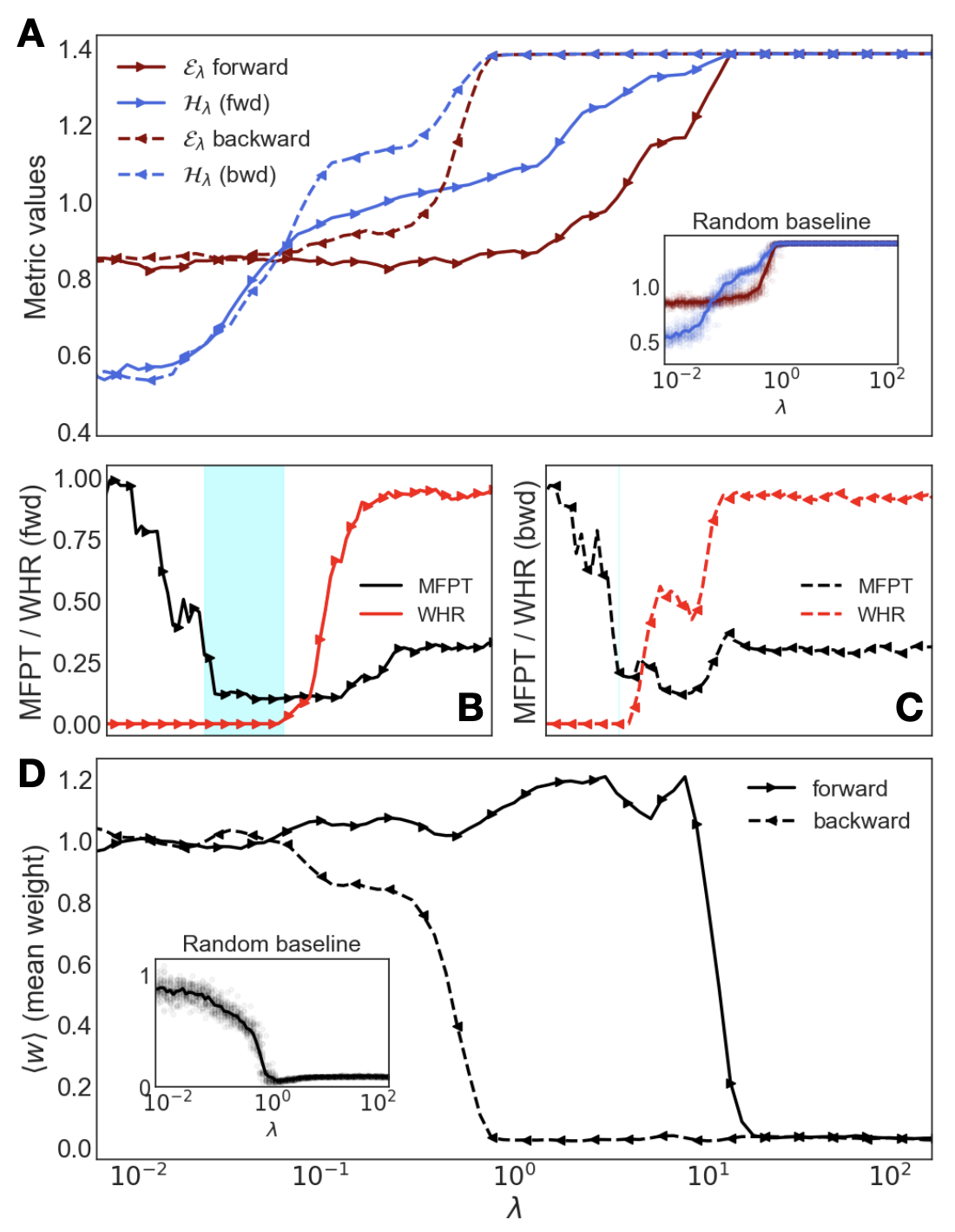
## Multi-Panel Scientific Plot: Metric Analysis vs. Parameter λ ### Overview The image is a composite figure containing four distinct plots (labeled A, B, C, D) that analyze the behavior of various metrics as a function of a parameter λ (lambda). The x-axis for all main plots is λ, presented on a logarithmic scale. The plots compare "forward" and "backward" processes or directions for different metrics. Insets in panels A and D show "Random baseline" comparisons. ### Components/Axes * **Panel A (Top):** * **Y-axis:** "Metric values" (linear scale, range ~0.4 to 1.4). * **X-axis:** λ (logarithmic scale, range 10⁻² to 10²). * **Legend (Top-Left):** * `ελ forward` (Solid dark red line, right-pointing triangle markers) * `Hλ (fwd)` (Solid blue line, right-pointing triangle markers) * `ελ backward` (Dashed dark red line, left-pointing triangle markers) * `Hλ (bwd)` (Dashed blue line, left-pointing triangle markers) * **Inset (Bottom-Right):** Titled "Random baseline". Y-axis range ~0.5 to 1.0. X-axis is λ (10⁻² to 10²). Shows two shaded bands (red and blue) representing baseline distributions. * **Panel B (Middle-Left):** * **Y-axis:** "MFPT / WHR (fwd)" (linear scale, range 0.00 to 1.00). * **X-axis:** λ (logarithmic scale, range 10⁻² to 10²). * **Legend (Center-Right):** * `MFPT` (Solid black line, no markers) * `WHR` (Solid red line, right-pointing triangle markers) * **Annotation:** A light cyan vertical shaded band spans approximately λ = 10⁻¹ to 10⁰. * **Panel C (Middle-Right):** * **Y-axis:** "MFPT / WHR (bwd)" (linear scale, range 0.00 to 1.00). * **X-axis:** λ (logarithmic scale, range 10⁻² to 10²). * **Legend (Center-Right):** * `MFPT` (Dashed black line, no markers) * `WHR` (Dashed red line, left-pointing triangle markers) * **Panel D (Bottom):** * **Y-axis:** "⟨w⟩ (mean weight)" (linear scale, range 0.0 to 1.2). * **X-axis:** λ (logarithmic scale, range 10⁻² to 10²). * **Legend (Top-Right):** * `forward` (Solid black line, right-pointing triangle markers) * `backward` (Dashed black line, left-pointing triangle markers) * **Inset (Bottom-Left):** Titled "Random baseline". Y-axis range 0 to 1. X-axis is λ (10⁻² to 10²). Shows a single shaded grey band. ### Detailed Analysis **Panel A: Metric Values (ελ and Hλ)** * **Trend Verification:** * `ελ forward` (Solid Red): Starts ~0.85, remains relatively flat with minor fluctuations until λ ≈ 10⁰, then increases sharply, plateauing near 1.4 for λ > 10¹. * `Hλ (fwd)` (Solid Blue): Starts lower at ~0.55, increases steadily across the entire λ range, approaching the 1.4 plateau near λ=10¹. * `ελ backward` (Dashed Red): Follows a similar shape to its forward counterpart but is shifted to the left (lower λ). It begins its sharp rise earlier, around λ=10⁻¹. * `Hλ (bwd)` (Dashed Blue): Also shifted left relative to its forward counterpart. It rises steeply between λ=10⁻² and 10⁻¹, reaching the plateau earlier than the forward Hλ. * **Key Data Points (Approximate):** * At λ=10⁻²: ελ fwd/bwd ≈ 0.85; Hλ fwd/bwd ≈ 0.55. * At λ=10⁰: ελ fwd ≈ 0.9, ελ bwd ≈ 1.3; Hλ fwd ≈ 1.05, Hλ bwd ≈ 1.35. * At λ=10¹: All four series converge near 1.4. * **Inset (Random Baseline):** Shows that for a random baseline, both metrics (red and blue bands) transition from lower to higher values around λ=10⁰, but the transition is less sharp and the final plateau is lower (~1.0) compared to the main plot. **Panels B & C: MFPT and WHR (Forward vs. Backward)** * **Trend Verification:** * **MFPT (Black lines):** In both forward (B, solid) and backward (C, dashed) plots, MFPT starts high (~1.0), drops sharply as λ increases from 10⁻² to ~10⁻¹, reaches a minimum, and then shows a slight, noisy recovery for higher λ. The minimum occurs within or near the cyan shaded region in B. * **WHR (Red lines):** In both plots, WHR starts near 0.0, remains low until λ ≈ 10⁻¹, then increases sharply, plateauing near 1.0 for λ > 10⁰. The rise is slightly more abrupt in the backward plot (C). * **Key Data Points (Approximate):** * At λ=10⁻²: MFPT ≈ 1.0; WHR ≈ 0.0. * At λ=10⁻¹ (within cyan band in B): MFPT ≈ 0.1-0.2; WHR begins its rise from ~0.0. * At λ=10⁰: MFPT ≈ 0.2-0.3; WHR ≈ 0.9-1.0. * At λ=10¹: MFPT ≈ 0.3; WHR ≈ 1.0. **Panel D: Mean Weight ⟨w⟩** * **Trend Verification:** * `forward` (Solid Black): Starts near 1.0, remains stable with minor fluctuations until λ ≈ 10¹, then drops precipitously to near 0.0. * `backward` (Dashed Black): Starts near 1.0, begins a steady decline earlier (around λ=10⁻¹), drops sharply to near 0.0 by λ=10⁰, and remains there. * **Key Data Points (Approximate):** * At λ=10⁻²: Both series ≈ 1.0. * At λ=10⁰: Forward ≈ 1.1, Backward ≈ 0.05. * At λ=10¹: Forward begins its sharp drop from ~1.2; Backward ≈ 0.0. * At λ=10²: Both series ≈ 0.0. * **Inset (Random Baseline):** Shows the mean weight for a random baseline starts near 1.0 and drops to near 0.0 around λ=10⁰, a transition point earlier than the forward process in the main plot but similar to the backward process. ### Key Observations 1. **Directional Asymmetry:** A consistent theme is that "backward" processes (dashed lines) undergo their characteristic transitions at lower λ values than their "forward" counterparts (solid lines). This is evident in all panels (A, C, D). 2. **Convergence at High λ:** In Panel A, all four metric series converge to the same high value (~1.4) for large λ. In Panels B and C, WHR converges to ~1.0, while MFPT stabilizes at a low but non-zero value. 3. **Critical Transition Zones:** The plots suggest critical λ ranges where system behavior changes dramatically: * λ ≈ 10⁻¹ to 10⁰: MFPT minimum and WHR rise (Panels B, C); Backward mean weight collapses (Panel D). * λ ≈ 10⁰ to 10¹: Forward metrics (ελ, Hλ) rise to plateau (Panel A); Forward mean weight collapses (Panel D). 4. **Baseline Comparison:** The insets show that the observed trends in the main plots deviate significantly from a "Random baseline," particularly in the sharpness of transitions and the final plateau values (e.g., Panel A inset vs. main plot). ### Interpretation This figure likely analyzes the performance or state of a system (e.g., a neural network, optimization process, or dynamical system) as a regularization or control parameter λ is varied. The "forward" and "backward" labels may refer to training vs. inference, two different algorithmic directions, or perturbation directions. * **What the data suggests:** The system undergoes phase-transition-like changes. At low λ, it appears to be in one state (high MFPT, low WHR, high mean weight). As λ increases, it transitions to a different state (low MFPT, high WHR, low mean weight). The "backward" process is more sensitive, transitioning at lower λ. * **Relationship between elements:** The metrics are correlated. The collapse of mean weight (Panel D) coincides with the rise of WHR and the fall of MFPT (Panels B, C). The rise of ελ and Hλ (Panel A) may represent increasing error or entropy as the system is pushed into a new regime by larger λ. * **Notable anomalies:** The slight recovery of MFPT at high λ (Panels B, C) is interesting and may indicate a secondary effect or noise. The fact that forward and backward mean weights collapse at different λ values (Panel D) is a key finding, suggesting hysteresis or path-dependence in the system's response to λ. * **Underlying message:** The parameter λ acts as a strong control knob. There is a critical region (around λ=1) where the system's fundamental behavior changes. The direction of traversal (forward/backward) matters significantly, indicating the system's landscape is non-symmetric or has memory. The deviation from the random baseline confirms the observed phenomena are specific to the structured system under study.