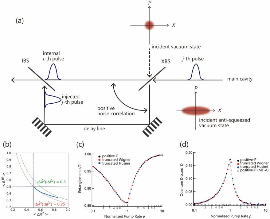
## Composite Figure: Quantum Optics Experiment and Simulation Results ### Overview The image presents a composite figure comprising a schematic diagram of a quantum optics experiment and three plots comparing simulation results obtained using different theoretical approaches. The experiment involves interacting pulses in a main cavity, and the simulations explore entanglement and quantum discord as a function of normalized pump rate. ### Components/Axes **Figure (a): Schematic Diagram** * **Title:** None explicitly stated, but it represents the experimental setup. * **Components:** * IBS (Input Beam Splitter): Located on the top-left. * XBS (Output Beam Splitter): Located on the top-right. * Main Cavity: The central region where the pulses interact. * Delay Line: At the bottom, connecting the output of IBS to the input of XBS. * Mirrors: Represented by parallel lines. * Pulses: "internal *i*-th pulse" and "injected *j*-th pulse" are shown as Gaussian-like curves. * Incident vacuum state: Shown as a red circle at the top, with axes labeled P and X. * Incident anti-squeezed vacuum state: Shown as a red ellipse at the bottom, with axes labeled P and X. * Positive noise correlation: Indicated by a curved arrow. **Figure (b): Plot of Variance Product** * **X-axis:** `<ΔX²>` (Variance of X) - Ranges from 0.2 to 1.0. * **Y-axis:** `<ΔP²>` (Variance of P) - Ranges from 0.2 to 1.0. * **Curves:** * `(ΔX²)(ΔP²) = 0.3`: Represented by a green dashed line. * `(ΔX²)(ΔP²) = 0.25`: Represented by a blue line. **Figure (c): Plot of Entanglement** * **X-axis:** Normalized Pump Rate *p* - Logarithmic scale from 0.1 to 10. * **Y-axis:** Entanglement ε/2 - Linear scale from 0.85 to 1.00. * **Data Series (Legend - top-right):** * positive-P: Black dots. * truncated Wigner: Red dots. * truncated Husimi: Blue dots. **Figure (d): Plot of Quantum Discord** * **X-axis:** Normalized Pump Rate *p* - Logarithmic scale from 0.1 to 10. * **Y-axis:** Quantum Discord *D* - Linear scale from 0.00 to 0.20. * **Data Series (Legend - top-right):** * positive-P: Black dots. * truncated Wigner: Red dots. * truncated Husimi: Blue dots. * positive-P (MF-A): White dots. ### Detailed Analysis **Figure (a): Schematic Diagram** The diagram illustrates an experimental setup involving two beam splitters (IBS and XBS) and a main cavity. Pulses are injected and interact within the cavity. The delay line provides feedback, and the incident states are either vacuum or anti-squeezed vacuum states. **Figure (b): Plot of Variance Product** The plot shows the relationship between the variances of X and P. The curves represent constant values of the product of these variances. The blue line is below the green line. * The blue line representing `(ΔX²)(ΔP²) = 0.25` starts at approximately `<ΔX²>` = 0.2, `<ΔP²>` = 0.8 and ends at `<ΔX²>` = 0.8, `<ΔP²>` = 0.3. * The green line representing `(ΔX²)(ΔP²) = 0.3` starts at approximately `<ΔX²>` = 0.2, `<ΔP²>` = 0.9 and ends at `<ΔX²>` = 0.9, `<ΔP²>` = 0.3. **Figure (c): Plot of Entanglement** The plot shows how entanglement (ε/2) varies with the normalized pump rate *p*. All three data series (positive-P, truncated Wigner, and truncated Husimi) exhibit a similar trend: * Initially, entanglement is high (close to 1.0) at low pump rates (around 0.1). * As the pump rate increases, entanglement decreases, reaching a minimum around *p* = 1. * Beyond *p* = 1, entanglement increases again, approaching 1.0 at high pump rates (around 10). * The minimum entanglement value is approximately 0.86 at p=1. **Figure (d): Plot of Quantum Discord** The plot shows how quantum discord *D* varies with the normalized pump rate *p*. The data series exhibit the following trends: * All data series start near 0 at low pump rates (around 0.1). * As the pump rate increases, quantum discord increases sharply, reaching a maximum around *p* = 1. * Beyond *p* = 1, quantum discord decreases, approaching 0 at high pump rates (around 10). * The maximum quantum discord value is approximately 0.18 at p=1. ### Key Observations * The schematic diagram illustrates the experimental setup for generating and manipulating quantum states of light. * The variance product plot shows the uncertainty relationship between the variances of X and P. * The entanglement plot shows that entanglement is high at both low and high pump rates, with a minimum around *p* = 1. * The quantum discord plot shows that quantum discord is maximized around *p* = 1 and approaches zero at both low and high pump rates. * The different theoretical approaches (positive-P, truncated Wigner, truncated Husimi, and positive-P (MF-A)) yield similar results for both entanglement and quantum discord, especially at low and high pump rates. ### Interpretation The data suggests that the normalized pump rate *p* plays a crucial role in determining the entanglement and quantum discord of the system. The observed trends indicate that there is an optimal pump rate (around *p* = 1) for maximizing quantum discord, while entanglement is generally high except around this optimal pump rate. The agreement between the different theoretical approaches suggests that the results are robust and not strongly dependent on the specific approximation used. The experiment and simulations demonstrate the generation and manipulation of non-classical states of light, which are essential for quantum information processing and quantum communication. The dip in entanglement and peak in quantum discord around p=1 may indicate a transition in the system's behavior or a change in the dominant physical processes.

\n ## Diagram: Quantum Optical Setup and Entanglement Analysis ### Overview The image presents a diagram of a quantum optical setup involving an intracavity beam splitter (IBS) and an external beam splitter (XBS), alongside three plots analyzing entanglement and quantum discord as a function of normalized pump rate. The setup appears designed to generate and analyze non-classical states of light. ### Components/Axes The diagram consists of four sub-images labeled (a), (b), (c), and (d). **(a) Quantum Optical Setup:** * **IBS:** Intracavity Beam Splitter. * **XBS:** External Beam Splitter. * **Main Cavity:** Represented by parallel lines. * **Incident Vacuum State:** Labeled above the XBS. * **Incident Anti-squeezed Vacuum State:** Labeled below the XBS. * **Internal i-th pulse:** Injected into the IBS. * **Injected j-th pulse:** Injected into the IBS. * **Delay Line:** Connecting the IBS and XBS. * **Positive Noise Correlation:** Arrow indicating correlation between pulses. * **P & X axes:** Representing momentum and position quadratures, shown as ellipses. **(b) Variance Plot:** * **X-axis:** `<ΔX²>` (approximately 0.2 to 1.0). * **Y-axis:** `V = Δ²P / <ΔX²>` (approximately 0.2 to 0.9). * **Curves:** Two curves are plotted, labeled with equations: `(ΔX²)(ΔP²) = 0.3` (green) and `(ΔX²)(ΔP²) = 0.25` (blue). **(c) Entanglement Plot:** * **X-axis:** Normalized Pump Rate ρ (approximately 0.1 to 10). * **Y-axis:** Entanglement E/2 (approximately 0.85 to 1.0). * **Curves:** Three curves are plotted: * positive-P (red) * truncated Wigner (blue) * truncated Husimi (black) **(d) Quantum Discord Plot:** * **X-axis:** Normalized Pump Rate ρ (approximately 0.1 to 10). * **Y-axis:** Quantum Discord D (approximately 0.0 to 0.2). * **Curves:** Three curves are plotted: * positive-P (red) * truncated Wigner (blue) * truncated Husimi (black) and positive-P (MF-A) (grey) ### Detailed Analysis or Content Details **(a) Quantum Optical Setup:** The setup involves injecting pulses into a cavity containing an intracavity beam splitter. The XBS splits the output, and the delay line introduces a time delay between the pulses. The diagram indicates a positive correlation between the noise in the pulses. The P and X axes represent the quadratures of the electromagnetic field. **(b) Variance Plot:** The green curve `(ΔX²)(ΔP²) = 0.3` starts at approximately V = 0.85 when `<ΔX²>` = 0.2, and decreases to approximately V = 0.3 when `<ΔX²>` = 1.0. The blue curve `(ΔX²)(ΔP²) = 0.25` starts at approximately V = 0.7 when `<ΔX²>` = 0.2, and decreases to approximately V = 0.25 when `<ΔX²>` = 1.0. Both curves exhibit a decreasing trend. **(c) Entanglement Plot:** All three curves (positive-P, truncated Wigner, truncated Husimi) start at approximately E/2 = 0.98 when ρ = 0.1. As ρ increases, all curves decrease. The positive-P curve (red) decreases more rapidly than the other two. At ρ = 10, the positive-P curve reaches approximately E/2 = 0.86, the truncated Wigner curve reaches approximately E/2 = 0.88, and the truncated Husimi curve reaches approximately E/2 = 0.90. **(d) Quantum Discord Plot:** The positive-P curve (red) starts at approximately D = 0.02 when ρ = 0.1 and increases to a peak of approximately D = 0.16 at ρ = 3. It then decreases to approximately D = 0.05 at ρ = 10. The truncated Wigner curve (blue) starts at approximately D = 0.01 when ρ = 0.1 and increases to a peak of approximately D = 0.12 at ρ = 3. It then decreases to approximately D = 0.03 at ρ = 10. The truncated Husimi curve (black) and positive-P (MF-A) (grey) are very close to zero across the entire range of ρ. ### Key Observations * The variance plot (b) shows an inverse relationship between the variances of the position and momentum quadratures, consistent with the uncertainty principle. * The entanglement plot (c) demonstrates that entanglement decreases as the normalized pump rate increases. * The quantum discord plot (d) shows that quantum discord initially increases with the pump rate, reaches a maximum, and then decreases. * The positive-P method appears to show the most significant decrease in entanglement with increasing pump rate. * The truncated Husimi and positive-P (MF-A) methods show minimal quantum discord. ### Interpretation The diagram illustrates a setup for generating and characterizing non-classical states of light. The plots reveal the interplay between entanglement and quantum discord as a function of the pump rate. The decrease in entanglement with increasing pump rate suggests that the system transitions from a highly entangled state to a more classical state. The behavior of quantum discord, which can be non-zero even in the absence of entanglement, indicates the presence of quantum correlations beyond entanglement. The differences between the curves obtained using different methods (positive-P, truncated Wigner, truncated Husimi) highlight the sensitivity of these measures to the specific state representation used. The setup and analysis likely aim to explore the limits of entanglement and quantum correlations in optical systems and to understand the role of noise and decoherence in these processes. The positive noise correlation is likely a key element in the dynamics of the system. The choice of the pump rate is critical in controlling the degree of entanglement and quantum discord.

## Quantum Optics Diagram and Associated Data Plots ### Overview The image is a composite technical figure containing four panels labeled (a) through (d). Panel (a) is a schematic diagram of an optical setup involving pulses and quantum states. Panels (b), (c), and (d) are quantitative plots showing relationships between quantum mechanical variables. The overall subject appears to be the analysis of quantum correlations (entanglement and discord) in a system involving optical pulses and squeezed states. ### Components/Axes **Panel (a): Optical Setup Diagram** * **Main Components:** * **Main Cavity:** A horizontal line representing the primary optical path. * **IBS & XBS:** Two beam splitters (likely "Input Beam Splitter" and "Output Beam Splitter") intersecting the main cavity. * **Delay Line:** A rectangular loop below the main cavity, connected to the IBS and XBS, containing two striped blocks (likely mirrors or phase shifters). * **Pulses:** Gaussian-shaped pulses labeled "internal i-th pulse" (on the main cavity), "injected j-th pulse" (entering the IBS from below), and "j-th pulse" (exiting the XBS to the right). * **Quantum States (Phase Space Representations):** * **Top Right:** A circular red blob on a P vs. X axis, labeled "incident vacuum state". * **Bottom Right:** An elliptical red blob on a P vs. X axis, labeled "incident anti-squeezed vacuum state". * **Annotations:** * A dashed arrow points from the "incident vacuum state" to the XBS. * A curved arrow labeled "positive noise correlation" points from the delay line back to the main cavity path between the IBS and XBS. **Panel (b): Uncertainty Relation Plot** * **X-axis:** `<ΔX²>` (Approximate variance of quadrature X). Scale: 0.2 to 1.0. * **Y-axis:** `<ΔP²>` (Approximate variance of quadrature P). Scale: 0.2 to 1.0. * **Data Series:** Two curves. * **Green Curve:** Labeled `(ΔX²)(ΔP²) = 0.3`. Starts high on the left, slopes downward to the right. * **Red Curve:** Labeled `(ΔX²)(ΔP²) = 0.25`. Starts higher than the green curve on the left, slopes downward more steeply, crossing below the green curve. * **Reference Lines:** A vertical dashed blue line at `<ΔX²> ≈ 0.5` and a horizontal dashed blue line at `<ΔP²> = 0.5`. **Panel (c): Entanglement vs. Pump Rate Plot** * **X-axis:** `Normalized Pump Rate p`. Logarithmic scale from 0.1 to 10. * **Y-axis:** `Entanglement E/2`. Linear scale from 0.85 to 1.00. * **Legend (Top Right):** * Black circles: `positive-P` * Red squares: `truncated Wigner` * Blue diamonds: `truncated Husimi` * **Data Trend:** All three series follow a distinct U-shaped curve. The value starts near 0.97 at p=0.1, decreases to a minimum of approximately 0.86 at p=1, and then increases back to near 1.00 at p=10. **Panel (d): Quantum Discord vs. Pump Rate Plot** * **X-axis:** `Normalized Pump Rate p`. Logarithmic scale from 0.1 to 10. * **Y-axis:** `Quantum Discord D`. Linear scale from 0.00 to 0.20. * **Legend (Top Right):** * Black circles: `positive-P` * Red squares: `truncated Wigner` * Blue diamonds: `truncated Husimi` * Open circles: `positive-P (MF-A)` * **Data Trend:** All series show a sharp peak. The value is near 0.00 at p=0.1, rises to a maximum of approximately 0.17 at p=1, and then falls back to near 0.00 at p=10. The `positive-P (MF-A)` series (open circles) follows the same trend but appears slightly lower at the peak. ### Detailed Analysis **Panel (b) Analysis:** The plot illustrates the Heisenberg uncertainty relation for two different constant products of variances. The green curve (`(ΔX²)(ΔP²) = 0.3`) represents a state with higher overall uncertainty than the red curve (`(ΔX²)(ΔP²) = 0.25`). The intersection of the curves with the dashed reference lines at (0.5, 0.5) shows that the state with the lower uncertainty product (red) can achieve a variance below 0.5 in one quadrature only at the expense of a variance significantly above 0.5 in the other, while the state with the higher product (green) has both variances above 0.5 at that point. **Panel (c) & (d) Cross-Reference:** The two plots share the same x-axis (`Normalized Pump Rate p`). There is a clear inverse relationship between the trends of Entanglement (E/2) and Quantum Discord (D). * At low pump rates (p < 1), Entanglement is high and decreasing, while Discord is low and increasing. * At the critical pump rate of **p = 1**, Entanglement reaches its **minimum** (~0.86) and Quantum Discord reaches its **maximum** (~0.17). * At high pump rates (p > 1), Entanglement increases back towards its initial value, while Discord decreases back towards zero. The three computational methods (`positive-P`, `truncated Wigner`, `truncated Husimi`) show excellent agreement across the entire range for both metrics, suggesting robustness in the results. The `positive-P (MF-A)` method in panel (d) shows a slightly lower discord peak. ### Key Observations 1. **Critical Point at p=1:** The system exhibits a distinct transition or resonance at a normalized pump rate of 1, marked by a minimum in entanglement and a maximum in quantum discord. 2. **Method Agreement:** The strong consistency between the three primary numerical methods (`positive-P`, `Wigner`, `Husimi`) in panels (c) and (d) validates the reported trends. 3. **Uncertainty Trade-off:** Panel (b) visually demonstrates the fundamental quantum trade-off between the uncertainties of conjugate variables (X and P), with different curves representing different levels of "squeezing" or state preparation. 4. **Diagrammatic Flow:** Panel (a) suggests a mechanism where an injected pulse (`j-th`) interacts with an internal pulse (`i-th`) via a delay line, creating a "positive noise correlation" that influences the output, with the system being probed by different incident quantum states (vacuum vs. anti-squeezed). ### Interpretation This figure collectively investigates the dynamics of quantum correlations in a driven optical system. The schematic in (a) proposes a physical setup where pulses are correlated via a delayed feedback loop. The data in (c) and (d) quantify how a control parameter—the pump rate—modulates the nature of these correlations. The central finding is the **complementary behavior of entanglement and quantum discord** around p=1. Entanglement, a stronger form of quantum correlation, is suppressed at the critical point, while quantum discord, which can exist even without entanglement, is maximized. This suggests a **transfer or conversion between different types of quantum correlations** as the system's drive strength changes. The system is most "quantum" in a different sense (high discord) precisely when it is least entangled. The uncertainty plot (b) provides foundational context, showing the type of non-classical states (squeezed states, where one variance is below the 0.5 limit) that are likely involved in the processes generating the correlations measured in (c) and (d). The anti-squeezed state shown in (a) corresponds to a point on one of these uncertainty curves. In essence, the figure demonstrates that by tuning the pump rate, one can navigate a landscape where quantum information is encoded either in strongly entangled states or in states with quantum discord but less entanglement, which has implications for quantum information processing protocols.

## Diagram: Quantum State Manipulation and Correlation Analysis ### Overview The image depicts a quantum optical setup for manipulating vacuum states and analyzing correlations between position (X) and momentum (P) quadratures. It includes a schematic diagram (a) and three graphs (b, c, d) showing relationships between quantum uncertainties, entanglement, and quantum discord as functions of pump rate. --- ### Components/Axes #### (a) Schematic Diagram - **Components**: - **Main cavity**: Right side, labeled with "incident vacuum state" (red ellipse) and "incident anti-squeezed vacuum state" (red ellipse with arrow). - **Delay line**: Horizontal line at the bottom, with striped patterns indicating phase shifts. - **IBS (Intra-Cavity Beam Splitter)**: Left side, with an incoming "internal i-th pulse" (blue curve). - **XBS (Crossed Beam Splitter)**: Center, with an outgoing "injected j-th pulse" (blue curve) and "positive noise correlation" (arrow). - **Pulses**: - "internal i-th pulse" (blue curve) above IBS. - "j-th pulse" (blue curve) above XBS. - **Axes**: - Horizontal axis labeled "X" (position). - Vertical axis labeled "P" (momentum). #### (b) Graph: Uncertainty Product vs. Position Uncertainty - **Axes**: - X-axis: `<ΔX̂²>` (position uncertainty squared), range 0.2–1.0. - Y-axis: `<ΔP̂²>` (momentum uncertainty squared), range 0.2–1.0. - **Curves**: - Green dashed line: `(ΔX̂²)(ΔP̂²) = 0.3`. - Red dashed line: `(ΔX̂²)(ΔP̂²) = 0.25`. - **Legend**: Located at bottom-left, associating colors with uncertainty products. #### (c) Graph: Entanglement vs. Normalized Pump Rate - **Axes**: - X-axis: Normalized Pump Rate `p` (log scale, 0.1–10). - Y-axis: Entanglement `ε/2`, range 0.85–1.0. - **Data Series**: - **Positive-P** (black dots): Peaks at `p=1`, drops to ~0.85 at `p=10`. - **Truncated Wigner** (red circles): Similar trend to Positive-P but slightly lower. - **Truncated Husimi** (blue squares): Smoother curve, peaks at `p=1`. - **Legend**: Top-right, associating markers with states. #### (d) Graph: Quantum Discord vs. Normalized Pump Rate - **Axes**: - X-axis: Normalized Pump Rate `p` (log scale, 0.1–10). - Y-axis: Quantum Discord `D`, range 0–0.2. - **Data Series**: - **Positive-P** (black dots): Peaks at `p=1` (~0.15). - **Truncated Wigner** (red circles): Similar peak but lower amplitude. - **Truncated Husimi** (blue squares): Lower peak (~0.1). - **Positive-P (MF-A)** (open circles): Overlaps with Positive-P but slightly lower. - **Legend**: Top-right, associating markers with states. --- ### Detailed Analysis #### (b) Uncertainty Product - The green and red curves represent the product of position and momentum uncertainties. As `<ΔX̂²>` increases, `<ΔP̂²>` decreases, consistent with quantum squeezing. The red curve (0.25) lies below the green curve (0.3), indicating tighter squeezing. #### (c) Entanglement - All states show maximum entanglement at `p=1`, with entanglement dropping as `p` increases. The Positive-P state maintains the highest entanglement across all pump rates. #### (d) Quantum Discord - Quantum Discord peaks at `p=1` for all states, with Positive-P (MF-A) showing the highest value. Discord decreases as `p` increases, suggesting reduced quantum correlations at higher pump rates. --- ### Key Observations 1. **Optimal Pump Rate**: All metrics (entanglement, discord) peak at `p=1`, indicating optimal quantum state manipulation at this pump rate. 2. **State Differences**: - Positive-P states exhibit higher entanglement and discord than truncated states. - Truncated Husimi states show smoother trends compared to truncated Wigner. 3. **Uncertainty Trade-off**: The uncertainty product curves in (b) confirm the Heisenberg limit, with squeezing achievable for specific pump rates. --- ### Interpretation The setup in (a) uses pulsed interactions to generate squeezed and entangled states from an incident vacuum. The graphs (b–d) quantify how pump rate affects quantum properties: - **Entanglement** and **quantum discord** are maximized at `p=1`, suggesting this is the optimal operating point for quantum information tasks. - The **Positive-P state** outperforms truncated states in both entanglement and discord, highlighting its utility for quantum communication. - The uncertainty product in (b) demonstrates that squeezing (reduced uncertainty product) is achievable, aligning with quantum optics principles. This analysis underscores the importance of pump rate optimization in quantum state engineering and the trade-offs between different quantum metrics.