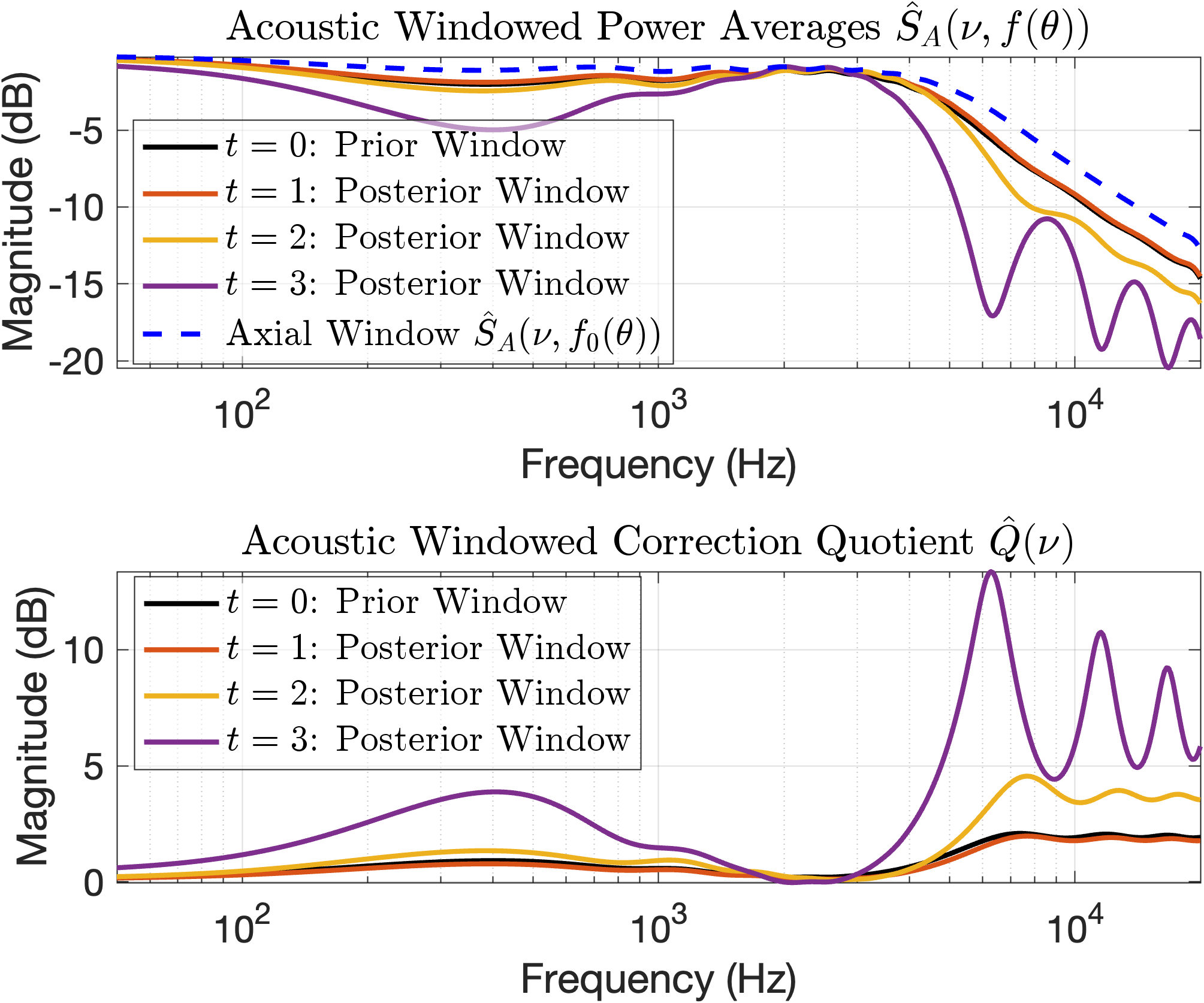
## Chart: Acoustic Windowed Power Averages and Correction Quotient ### Overview The image contains two line charts displaying acoustic windowed power averages and correction quotients as a function of frequency. The top chart shows the power averages for different time windows (prior, posterior, and axial), while the bottom chart shows the corresponding correction quotients. The x-axis represents frequency in Hz (logarithmic scale), and the y-axis represents magnitude in dB. ### Components/Axes **Top Chart:** * **Title:** Acoustic Windowed Power Averages Ŝ_A(ν, f(θ)) * **X-axis:** Frequency (Hz), logarithmic scale with markers at 10², 10³, and 10⁴. * **Y-axis:** Magnitude (dB), linear scale with markers from -20 to 0 in increments of 5 (-20, -15, -10, -5, 0). * **Legend (Top-Left):** * Black: t = 0: Prior Window * Orange: t = 1: Posterior Window * Yellow: t = 2: Posterior Window * Purple: t = 3: Posterior Window * Blue Dashed: Axial Window Ŝ_A(ν, f₀(θ)) **Bottom Chart:** * **Title:** Acoustic Windowed Correction Quotient Q̂(ν) * **X-axis:** Frequency (Hz), logarithmic scale with markers at 10², 10³, and 10⁴. * **Y-axis:** Magnitude (dB), linear scale with markers from 0 to 10 in increments of 5 (0, 5, 10). * **Legend (Top-Left):** * Black: t = 0: Prior Window * Orange: t = 1: Posterior Window * Yellow: t = 2: Posterior Window * Purple: t = 3: Posterior Window ### Detailed Analysis **Top Chart: Acoustic Windowed Power Averages** * **Black (t=0: Prior Window):** The line starts at approximately -2 dB, remains relatively flat until around 10³ Hz, and then decreases gradually to approximately -3 dB at 10⁴ Hz. * **Orange (t=1: Posterior Window):** The line starts at approximately -2 dB, remains relatively flat until around 10³ Hz, and then decreases to approximately -14 dB at 10⁴ Hz. * **Yellow (t=2: Posterior Window):** The line starts at approximately -2 dB, remains relatively flat until around 10³ Hz, and then decreases, reaching a minimum of approximately -17 dB around 5*10³ Hz, before increasing slightly to approximately -15 dB at 10⁴ Hz. * **Purple (t=3: Posterior Window):** The line starts at approximately -2 dB, remains relatively flat until around 10³ Hz, and then decreases significantly, reaching a minimum of approximately -21 dB around 4*10³ Hz, before oscillating to approximately -16 dB at 10⁴ Hz. * **Blue Dashed (Axial Window):** The line starts at approximately -1 dB, remains relatively flat until around 10³ Hz, and then decreases to approximately -10 dB at 10⁴ Hz. **Bottom Chart: Acoustic Windowed Correction Quotient** * **Black (t=0: Prior Window):** The line starts at approximately 1 dB, remains relatively flat until around 10³ Hz, and then increases slightly to approximately 2 dB at 10⁴ Hz. * **Orange (t=1: Posterior Window):** The line starts at approximately 1 dB, remains relatively flat until around 10³ Hz, and then increases slightly to approximately 3 dB at 10⁴ Hz. * **Yellow (t=2: Posterior Window):** The line starts at approximately 1 dB, remains relatively flat until around 10³ Hz, and then increases to approximately 4 dB at 10⁴ Hz. * **Purple (t=3: Posterior Window):** The line starts at approximately 1 dB, increases significantly after 10³ Hz, reaching a maximum of approximately 12 dB around 4*10³ Hz, before oscillating to approximately 7 dB at 10⁴ Hz. ### Key Observations * In the top chart, the power averages for all windows are similar at lower frequencies (around 10² Hz). * As frequency increases, the power averages for the posterior windows (t=1, t=2, t=3) and the axial window decrease more significantly than the prior window (t=0). * In the bottom chart, the correction quotients for the prior and posterior windows (t=0, t=1, t=2) are relatively flat and close to 0 dB until around 10³ Hz. * The correction quotient for t=3 increases significantly with frequency, indicating a larger correction is needed for this window at higher frequencies. ### Interpretation The charts illustrate the effect of different windowing techniques on acoustic power averages and the corresponding correction quotients. The prior window (t=0) appears to be less affected by frequency changes compared to the posterior windows (t=1, t=2, t=3) and the axial window. The correction quotient for t=3 suggests that this window requires a more substantial correction at higher frequencies, possibly due to increased distortion or noise. The data suggests that the choice of windowing technique can significantly impact the accuracy of acoustic measurements, especially at higher frequencies.