## Diagram: Expert Selection Process ### Overview The image is a diagram illustrating a three-step process for expert selection. It starts with a hidden token input, calculates similarity scores, transforms these into probabilities, and then selects the top-K experts. ### Components/Axes * **Operation 1: Similarity Score Calculation** * Formula: lₜ = uₜWₑc * Input: Hidden Token Input (u ∈ Rᴰ) * Process: Linear Projection * Matrix: Wₑc ∈ Rᴰˣᴺ * Expert Centroid Space (Weight-Space): Represented by a neural network diagram. * **Operation 2: Probability Transformation** * Input: Expert Logits (l ∈ Rᴺ) * Process: Softmax (sₜ = softmax(lₜ)) * Output: Expert Selection Probability (s ∈ Rᴺ) * Expert Logit Space (Latent-Space): Represented by a 3D Gaussian-like shape. * **Operation 3: Top-K Selection** * Input: Expert Selection Probability (s ∈ Rᴺ) * Process: Top-K selection * Output: Selected Experts (Sₜ) * Expert Selection Space (Decision-Space): Represented by a bar chart. ### Detailed Analysis * **Hidden Token Input:** A column of 8 gray boxes, representing the input vector u ∈ Rᴰ. * **Linear Projection:** A matrix with N columns, each column represented by a different color (orange, pink, light blue, green, light green, purple, gray). Each column has multiple dots, suggesting a high dimensionality. * **Expert Logits:** A column of N boxes, each corresponding to an expert. The boxes are colored similarly to the columns in the Linear Projection matrix. * **Softmax:** A box labeled "Softmax" representing the softmax function. * **Expert Selection Probability:** A bar chart with N bars, representing the probability of each expert being selected. The bars are in shades of blue, with the tallest bar being dark blue. * **Top-K Selection:** A box labeled "Top-K" representing the top-K selection process. * **Selected Experts:** A column of boxes, some filled with a dark green color, representing the selected experts Sₜ. ### Key Observations * The diagram illustrates a clear flow from input to selected experts. * The color-coding in the Linear Projection and Expert Logits suggests a correspondence between the experts and the columns in the matrix. * The Softmax function transforms the logits into probabilities, which are then used for expert selection. * The Expert Selection Space (Decision-Space) visually represents the selection process. ### Interpretation The diagram depicts a mechanism for selecting experts based on the similarity between a hidden token input and expert centroids. The process involves calculating similarity scores through linear projection, transforming these scores into probabilities using the softmax function, and then selecting the top-K experts based on these probabilities. The diagram highlights the transformation of the input from a high-dimensional space (Rᴰ) to a probability distribution over experts (Rᴺ), ultimately leading to the selection of a subset of experts (Sₜ). The use of different spaces (Weight-Space, Latent-Space, Decision-Space) suggests a multi-faceted approach to expert representation and selection.

\n ## Diagram: Mixture of Experts (MoE) System Flow ### Overview The image depicts a diagram illustrating the flow of data through a Mixture of Experts (MoE) system. The system consists of three main operations: Similarity Score Calculation, Probability Transformation, and Top-K Selection. The diagram shows how a hidden token input is processed through a linear projection to generate expert logits, which are then transformed into probabilities, and finally used to select a subset of experts. ### Components/Axes The diagram is segmented into three main operational blocks, labeled "Operation 1: Similarity Score Calculation", "Operation 2: Probability Transformation", and "Operation 3: Top-K Selection". Each block contains several components: * **Hidden Token Input:** Represented as `u ∈ R^d` (a vector in d-dimensional space). * **Linear Projection:** Depicted as a matrix multiplication with `W_l ∈ R^(d x P)` where P is the number of experts. * **Expert Logits:** Represented as `l ∈ R^P`. * **Expert Selection Probability:** Represented as `s_i = softmax(l)` and `s ∈ R^P`. * **Selected Experts:** Represented as `S_i`. * **Expert Centroid Space (Weight-Space):** A scatter plot showing expert centroids. * **Expert Logit Space (Latent-Space):** A visual representation of the expert logits. * **Expert Selection Space (Decision-Space):** A bar chart representing the expert selection probabilities. The diagram also includes mathematical equations: * `l_i = u_i * W_l` (Similarity Score Calculation) * `s_i = softmax(l)` (Probability Transformation) ### Detailed Analysis / Content Details The diagram illustrates a data flow from left to right. 1. **Operation 1: Similarity Score Calculation:** A hidden token input `u ∈ R^d` (represented as a vertical stack of numbers) is linearly projected using a weight matrix `W_l ∈ R^(d x P)` (represented as colored vertical bars). This results in expert logits `l ∈ R^P`. The colors of the bars in `W_l` are: yellow, orange, light blue, dark blue, green. The expert centroid space (Weight-Space) shows a scatter plot of expert centroids, with points clustered in different regions. 2. **Operation 2: Probability Transformation:** The expert logits `l` are passed through a softmax function to generate expert selection probabilities `s_i = softmax(l)`, represented as `s ∈ R^P`. This is visually depicted as a bar chart in the "Expert Selection Space (Decision-Space)". The bar chart shows varying probabilities for each expert. 3. **Operation 3: Top-K Selection:** A "Top-K" operation selects the top K experts based on their probabilities. The selected experts `S_i` are represented as a vertical stack of colored blocks, with the colors corresponding to the experts selected. The arrow indicates that only a subset of experts are chosen. The diagram uses dotted arrows to indicate the flow of data between operations. ### Key Observations * The system uses a linear projection to map the hidden token input to the expert logit space. * The softmax function is used to convert logits into probabilities, representing the relevance of each expert. * The Top-K selection mechanism allows the system to focus on a subset of experts for each input. * The diagram highlights the transformation of data from the input space to the latent space and then to the decision space. ### Interpretation The diagram illustrates a key component of Mixture of Experts models, which aim to improve model capacity and performance by dividing the task among multiple experts. The MoE architecture allows the model to specialize in different aspects of the data, leading to more efficient and accurate predictions. The diagram demonstrates how the input is routed to the most relevant experts based on a similarity score and a probability distribution. The Top-K selection ensures that only a limited number of experts are activated for each input, reducing computational cost. The visual representation of the different spaces (Weight-Space, Latent-Space, Decision-Space) provides a clear understanding of the data transformation process within the MoE system. The diagram is a conceptual illustration and does not contain specific numerical data, but rather focuses on the functional flow and mathematical operations involved.

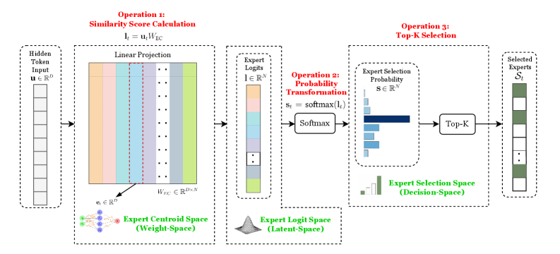
## Process Flow Diagram: Expert Selection Mechanism ### Overview This image is a technical process flow diagram illustrating a three-step mechanism for selecting "experts" (likely in a machine learning or neural network context, such as a Mixture-of-Experts model). The flow proceeds from left to right, starting with a "Hidden Token Input" and culminating in "Selected Experts." The diagram uses mathematical notation, color-coded blocks, and labeled spaces to explain the transformation of data. ### Components/Axes The diagram is segmented into four main vertical sections, connected by arrows indicating data flow. Each major operation is enclosed in a dashed box and labeled in red text. **1. Input (Far Left):** * **Label:** `Hidden Token Input` * **Mathematical Notation:** `u ∈ R^d` (indicating a vector `u` in a d-dimensional real space). * **Visual:** A vertical column of 8 empty white rectangles, representing a sequence of token vectors. **2. Operation 1: Similarity Score Calculation (Left-Center):** * **Title (Red):** `Operation 1: Similarity Score Calculation` * **Equation:** `l_i = u_i W_EC` * **Process Label:** `Linear Projection` * **Visual:** A large block composed of 8 vertical colored bars (from left to right: orange, light blue, purple, grey, light green, dark blue, yellow, dark green). These represent the projection of the input `u` onto expert centroids. * **Key Components:** * `W_EC ∈ R^(d×N)`: The weight matrix for the Expert Centroid Space. * `e_i ∈ R^d`: A single expert centroid vector, pointed to by an arrow from the colored bars. * **Space Label (Green, Bottom):** `Expert Centroid Space (Weight-Space)`. This is accompanied by a small diagram of interconnected nodes (green and blue dots). **3. Intermediate Output & Operation 2: Probability Transformation (Center):** * **Output Label:** `Expert Logits` * **Mathematical Notation:** `l ∈ R^N` (a vector of N logits). * **Visual:** A vertical column of 8 colored rectangles (matching the colors from the Linear Projection block), representing the raw similarity scores (logits) for each expert. * **Title (Red):** `Operation 2: Probability Transformation` * **Equation:** `s_i = softmax(l_i)` * **Process Label:** `Softmax` * **Space Label (Green, Bottom):** `Expert Logit Space (Latent-Space)`. This is accompanied by a small bell curve icon. **4. Operation 3: Top-K Selection & Output (Right):** * **Title (Red):** `Operation 3: Top-K Selection` * **Process Label:** `Top-K` * **Visual (Expert Selection Probability):** A horizontal bar chart labeled `Expert Selection Probability` with notation `s ∈ R^N`. It shows 8 bars of varying lengths. The 4th bar (dark blue) is the longest, followed by the 1st (orange) and 6th (dark green). The others are shorter. * **Space Label (Green, Bottom):** `Expert Selection Space (Decision-Space)`. This is accompanied by a small bar chart icon. * **Final Output Label:** `Selected Experts` * **Mathematical Notation:** `S_k` * **Visual:** A vertical column of 8 rectangles. The 1st (orange), 4th (dark blue), and 6th (dark green) are filled with a solid dark green color, indicating they are the "selected" experts from the Top-K operation. The other five are empty white rectangles. ### Detailed Analysis The diagram details a precise mathematical pipeline: 1. **Input Transformation:** A hidden token vector `u` is linearly projected using a weight matrix `W_EC` to produce a set of similarity scores or "logits" (`l`). Each logit corresponds to an expert, represented by a centroid `e_i` in the "Weight-Space." 2. **Probability Conversion:** The logits `l` are passed through a softmax function to convert them into a probability distribution `s`. This transforms the data from the "Latent-Space" (logits) to the "Decision-Space" (selection probabilities). 3. **Expert Selection:** A Top-K operation is applied to the probability distribution `s`. This selects the `k` experts with the highest selection probabilities. In the visual example, K appears to be 3, as three experts (1st, 4th, and 6th) are highlighted in the final "Selected Experts" block. ### Key Observations * **Color Consistency:** The color coding is consistent throughout the flow. The 4th expert (dark blue) has the highest logit, the highest selection probability, and is selected. The 1st (orange) and 6th (dark green) experts are also selected, corresponding to the next highest probabilities. * **Spatial Organization:** The diagram clearly segregates conceptual spaces: Weight-Space (where expert definitions live), Latent-Space (raw model outputs), and Decision-Space (final routing choices). * **Mathematical Rigor:** Every step is accompanied by its formal mathematical operation (`l_i = u_i W_EC`, `softmax`, `Top-K`), making the process unambiguous for a technical audience. * **Visual Example:** The bar chart for "Expert Selection Probability" provides a concrete example of the softmax output, and the final "Selected Experts" block shows the discrete outcome of the Top-K selection. ### Interpretation This diagram explains the **routing mechanism** in a Mixture-of-Experts (MoE) neural network layer. It answers the question: "Given an input token, how does the model decide which specialized sub-networks (experts) should process it?" * **What it demonstrates:** The process is a learned, dynamic routing system. Instead of sending every input to every expert (computationally expensive), the model uses a lightweight "gating network" (the operations shown) to compute a similarity score between the input and each expert's prototype (centroid). It then probabilistically selects only the most relevant experts (Top-K) for that specific input. * **Relationships:** The "Expert Centroid Space" (`W_EC`) contains the learned knowledge of what each expert specializes in. The input `u` is compared against these specializations. The softmax ensures the selection is a competition, and the Top-K enforces sparsity for efficiency. * **Significance:** This mechanism allows models to have a very large total number of parameters (many experts) while only activating a small subset for any given input, enabling scaling without a proportional increase in computational cost. The diagram meticulously breaks down the core computation that makes this efficient scaling possible.

## Diagram: Expert Selection Process in a Mixture of Experts Model ### Overview This diagram illustrates a three-stage process for selecting experts in a Mixture of Experts (MoE) architecture. It shows how input tokens are transformed through linear projections, probability calculations, and final expert selection. The process involves three key spaces: Weight-Space (Expert Centroid Space), Latent-Space (Expert Logit Space), and Decision-Space (Expert Selection Space). ### Components/Axes 1. **Input**: Hidden Token Input vector **u** ∈ ℝ^D 2. **Operation 1: Similarity Score Calculation** - Linear Projection: **l**_i = **u**_iW_IC - Visualized as a matrix with colored columns (orange, blue, green, etc.) 3. **Operation 2: Probability Transformation** - Softmax function: **s**_t = softmax(**l**_i) - Expert Logits visualized as a color gradient (pink to gray) 4. **Operation 3: Top-K Selection** - Expert Selection Space (Decision-Space) with probability bars - Top-K Selected Experts output **Legend Colors**: - Orange: Expert 1 - Blue: Expert 2 - Green: Expert 3 - Purple: Expert 4 - Gray: Expert 5 - Pink: High logit values - Dark Gray: Low logit values ### Detailed Analysis 1. **Similarity Score Calculation** - Input vector **u** is linearly projected through weight matrix W_IC - Produces similarity scores **l**_i for each expert - Visualized as vertical bars with varying heights (expert 1 has highest score) 2. **Probability Transformation** - Softmax converts logits to probabilities (0-1 range) - Probability distribution shows expert 1 with highest probability (~0.4) - Other experts have progressively lower probabilities 3. **Top-K Selection** - Top-K experts selected based on probability distribution - Visualized as selected experts (experts 1 and 2 in this case) - Remaining experts excluded from final selection ### Key Observations 1. Expert 1 consistently has the highest similarity score and probability 2. Probability distribution follows a clear decay pattern across experts 3. Top-K selection creates a binary decision space (selected vs excluded) 4. Color coding maintains consistency across all three operations ### Interpretation This diagram demonstrates how MoE models dynamically route input tokens to specialized experts. The process shows: 1. **Weight-Space** transformations create expert-specific representations 2. **Latent-Space** logits quantify expert relevance 3. **Decision-Space** makes final selection based on probability thresholds The softmax normalization ensures probabilistic interpretation of expert selection, while Top-K introduces sparsity in expert usage. This architecture enables efficient computation by activating only relevant experts for each input, balancing model capacity and computational efficiency. The consistent dominance of Expert 1 suggests potential issues with expert diversity or imbalance in the current configuration. A healthy MoE system would typically show more balanced expert utilization across different input types.