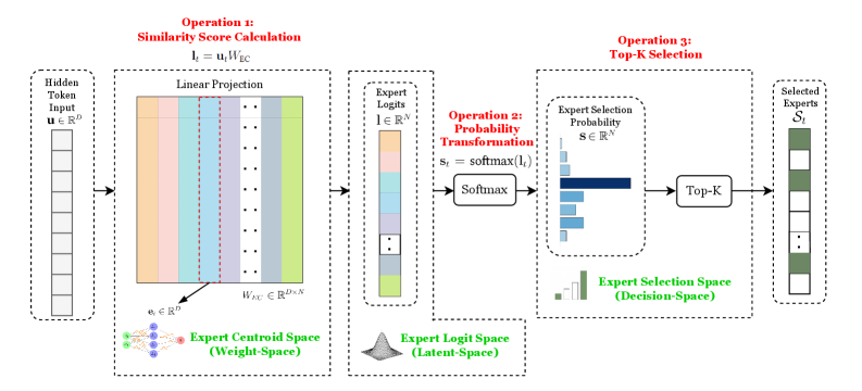
## Diagram: Expert Selection Process in a Mixture of Experts Model ### Overview This diagram illustrates a three-stage process for selecting experts in a Mixture of Experts (MoE) architecture. It shows how input tokens are transformed through linear projections, probability calculations, and final expert selection. The process involves three key spaces: Weight-Space (Expert Centroid Space), Latent-Space (Expert Logit Space), and Decision-Space (Expert Selection Space). ### Components/Axes 1. **Input**: Hidden Token Input vector **u** ∈ ℝ^D 2. **Operation 1: Similarity Score Calculation** - Linear Projection: **l**_i = **u**_iW_IC - Visualized as a matrix with colored columns (orange, blue, green, etc.) 3. **Operation 2: Probability Transformation** - Softmax function: **s**_t = softmax(**l**_i) - Expert Logits visualized as a color gradient (pink to gray) 4. **Operation 3: Top-K Selection** - Expert Selection Space (Decision-Space) with probability bars - Top-K Selected Experts output **Legend Colors**: - Orange: Expert 1 - Blue: Expert 2 - Green: Expert 3 - Purple: Expert 4 - Gray: Expert 5 - Pink: High logit values - Dark Gray: Low logit values ### Detailed Analysis 1. **Similarity Score Calculation** - Input vector **u** is linearly projected through weight matrix W_IC - Produces similarity scores **l**_i for each expert - Visualized as vertical bars with varying heights (expert 1 has highest score) 2. **Probability Transformation** - Softmax converts logits to probabilities (0-1 range) - Probability distribution shows expert 1 with highest probability (~0.4) - Other experts have progressively lower probabilities 3. **Top-K Selection** - Top-K experts selected based on probability distribution - Visualized as selected experts (experts 1 and 2 in this case) - Remaining experts excluded from final selection ### Key Observations 1. Expert 1 consistently has the highest similarity score and probability 2. Probability distribution follows a clear decay pattern across experts 3. Top-K selection creates a binary decision space (selected vs excluded) 4. Color coding maintains consistency across all three operations ### Interpretation This diagram demonstrates how MoE models dynamically route input tokens to specialized experts. The process shows: 1. **Weight-Space** transformations create expert-specific representations 2. **Latent-Space** logits quantify expert relevance 3. **Decision-Space** makes final selection based on probability thresholds The softmax normalization ensures probabilistic interpretation of expert selection, while Top-K introduces sparsity in expert usage. This architecture enables efficient computation by activating only relevant experts for each input, balancing model capacity and computational efficiency. The consistent dominance of Expert 1 suggests potential issues with expert diversity or imbalance in the current configuration. A healthy MoE system would typically show more balanced expert utilization across different input types.