## Chart: 2D φ⁴ Nearest Neighbours
### Overview
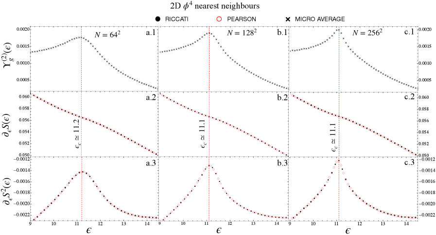
The image presents a series of line plots illustrating the behavior of different functions with respect to a variable epsilon (ε). The plots are arranged in a 3x3 grid, with each column representing a different value of N (64², 128², 256²). Each row represents a different function: Yg^(2)(ε), ∂εS(ε), and ∂εS²(ε). The plots compare results from RICCATI, PEARSON, and MICRO AVERAGE methods.
### Components/Axes
* **Title:** 2D φ⁴ nearest neighbours
* **Legend:** Located at the top of the image.
* Black filled circle: RICCATI
* Red open circle: PEARSON
* Black cross: MICRO AVERAGE
* **X-axis:** ε (epsilon), ranging from approximately 9 to 14 in all subplots.
* **Y-axes:**
* Top row (a.1, b.1, c.1): Yg^(2)(ε), ranging from approximately -0.001 to 0.002.
* Middle row (a.2, b.2, c.2): ∂εS(ε), ranging from approximately 0.050 to 0.060.
* Bottom row (a.3, b.3, c.3): ∂εS²(ε), ranging from approximately -0.0022 to -0.0012.
* **Vertical dashed red lines:** Indicate critical values εc, approximately equal to 11.2 for N=64², and 11.1 for N=128² and N=256².
* **Subplot labels:** a.1, a.2, a.3, b.1, b.2, b.3, c.1, c.2, c.3, located at the right of each subplot.
* **N values:** N = 64², N = 128², N = 256², located at the top of each column.
### Detailed Analysis
**Column 1: N = 64²**
* **a.1: Yg^(2)(ε):** The MICRO AVERAGE data (black crosses) starts at approximately 0.0013 at ε=9, increases to a peak of approximately 0.0018 at ε=11.2, and then decreases to approximately 0.0003 at ε=14.
* **a.2: ∂εS(ε):** The RICCATI (black filled circles) and PEARSON (red open circles) data are almost perfectly overlapping. The data decreases linearly from approximately 0.060 at ε=9 to approximately 0.050 at ε=14.
* **a.3: ∂εS²(ε):** The RICCATI (black filled circles) and PEARSON (red open circles) data are almost perfectly overlapping. The data forms a peak centered around ε=11.2, rising from approximately -0.0022 at ε=9 to approximately -0.0014 at ε=11.2, and then decreasing back to approximately -0.0022 at ε=14.
**Column 2: N = 128²**
* **b.1: Yg^(2)(ε):** The MICRO AVERAGE data (black crosses) starts at approximately 0.0013 at ε=9, increases to a peak of approximately 0.0019 at ε=11.1, and then decreases to approximately 0.0002 at ε=14.
* **b.2: ∂εS(ε):** The RICCATI (black filled circles) and PEARSON (red open circles) data are almost perfectly overlapping. The data decreases linearly from approximately 0.060 at ε=9 to approximately 0.050 at ε=14.
* **b.3: ∂εS²(ε):** The RICCATI (black filled circles) and PEARSON (red open circles) data are almost perfectly overlapping. The data forms a peak centered around ε=11.1, rising from approximately -0.0022 at ε=9 to approximately -0.0013 at ε=11.1, and then decreasing back to approximately -0.0022 at ε=14.
**Column 3: N = 256²**
* **c.1: Yg^(2)(ε):** The MICRO AVERAGE data (black crosses) starts at approximately 0.0014 at ε=9, increases to a peak of approximately 0.0020 at ε=11.1, and then decreases to approximately -0.0004 at ε=14.
* **c.2: ∂εS(ε):** The RICCATI (black filled circles) and PEARSON (red open circles) data are almost perfectly overlapping. The data decreases linearly from approximately 0.060 at ε=9 to approximately 0.050 at ε=14.
* **c.3: ∂εS²(ε):** The RICCATI (black filled circles) and PEARSON (red open circles) data are almost perfectly overlapping. The data forms a peak centered around ε=11.1, rising from approximately -0.0022 at ε=9 to approximately -0.0012 at ε=11.1, and then decreasing back to approximately -0.0022 at ε=14.
### Key Observations
* The RICCATI and PEARSON methods produce nearly identical results for ∂εS(ε) and ∂εS²(ε) across all values of N.
* The peak in Yg^(2)(ε) and ∂εS²(ε) becomes more pronounced and shifts slightly to the left as N increases.
* The linear decrease in ∂εS(ε) is consistent across all values of N.
* The vertical dashed lines indicate a critical value εc, which appears to be related to the peak in Yg^(2)(ε) and ∂εS²(ε).
### Interpretation
The plots compare the behavior of different functions related to a 2D φ⁴ model using different computational methods (RICCATI, PEARSON, and MICRO AVERAGE). The parameter N seems to represent a system size or resolution, and epsilon (ε) is a variable that influences the behavior of the functions.
The near-identical results from the RICCATI and PEARSON methods suggest that they are converging to the same solution for the given functions. The MICRO AVERAGE method provides a different perspective, particularly in the Yg^(2)(ε) plots, where it shows a distinct peak.
The shift and sharpening of the peaks in Yg^(2)(ε) and ∂εS²(ε) as N increases suggest that the system's behavior becomes more defined and potentially approaches a critical point or phase transition. The vertical lines at εc indicate a critical value of epsilon, which may be related to this transition.
The linear decrease in ∂εS(ε) suggests a consistent relationship between epsilon and this function, regardless of the value of N or the computational method used.