## Chart/Diagram: 2D $\phi^4$ nearest neighbours
### Overview
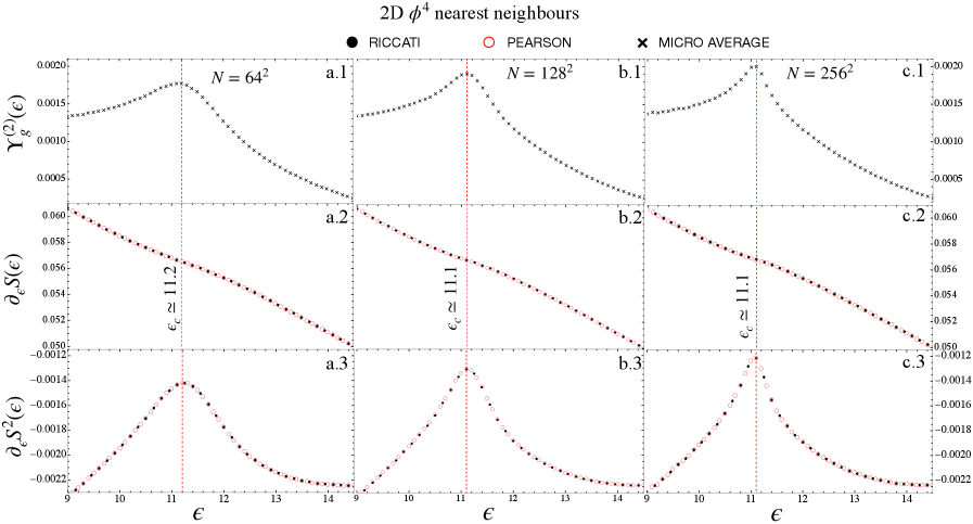
This image presents a 3x3 grid of plots analyzing the behavior of a 2D $\phi^4$ model across three different system sizes ($N = 64^2$, $N = 128^2$, and $N = 256^2$). The columns represent the system size, while the rows represent three different physical quantities: $\Upsilon_g^{(2)}(\epsilon)$, $\partial_\epsilon S(\epsilon)$, and $\partial_\epsilon S^2(\epsilon)$. The plots investigate the behavior of these quantities as a function of $\epsilon$ (ranging from 9 to 15), highlighting a critical value $\epsilon_c$.
### Components/Axes
* **Legend (Top Center):**
* **RICCATI:** Represented by black filled circles ($\bullet$).
* **PEARSON:** Represented by red open circles ($\circ$).
* **MICRO AVERAGE:** Represented by black crosses ($\times$).
* **Columns (System Size $N$):**
* **Left Column:** $N = 64^2$ (labeled a.1, a.2, a.3).
* **Middle Column:** $N = 128^2$ (labeled b.1, b.2, b.3).
* **Right Column:** $N = 256^2$ (labeled c.1, c.2, c.3).
* **Rows (Quantities):**
* **Top Row:** Y-axis labeled $\Upsilon_g^{(2)}(\epsilon)$. Scale: 0.0005 to 0.0020.
* **Middle Row:** Y-axis labeled $\partial_\epsilon S(\epsilon)$. Scale: 0.050 to 0.060.
* **Bottom Row:** Y-axis labeled $\partial_\epsilon S^2(\epsilon)$. Scale: -0.0022 to -0.0012.
* **X-Axis:** Labeled $\epsilon$ at the bottom of the grid. Range: 9 to 15.
* **Vertical Markers:** A red dashed vertical line is present in all plots, indicating the critical value $\epsilon_c$.
* Left column: $\epsilon_c \simeq 11.2$.
* Middle and Right columns: $\epsilon_c \simeq 11.1$.
### Detailed Analysis
#### Row 1: $\Upsilon_g^{(2)}(\epsilon)$ (Plots a.1, b.1, c.1)
* **Trend:** All plots show a sharp peak at $\epsilon_c$. The curve rises from $\epsilon=9$, peaks at $\epsilon_c$, and decays as $\epsilon$ increases toward 15.
* **Data Series:** Only "MICRO AVERAGE" (black crosses) is plotted.
* **Observation:** As the system size $N$ increases from $64^2$ to $256^2$, the peak becomes progressively sharper and higher, characteristic of finite-size scaling near a phase transition.
#### Row 2: $\partial_\epsilon S(\epsilon)$ (Plots a.2, b.2, c.2)
* **Trend:** All plots show a monotonic downward slope as $\epsilon$ increases.
* **Data Series:** Both "RICCATI" (black filled circles) and "PEARSON" (red open circles) are plotted.
* **Observation:** The two data series overlap almost perfectly across all three system sizes, indicating high consistency between the Riccati and Pearson methods. The red dashed line at $\epsilon_c$ intersects the curve at a point that appears to be an inflection point or a specific reference value.
#### Row 3: $\partial_\epsilon S^2(\epsilon)$ (Plots a.3, b.3, c.3)
* **Trend:** All plots show a peak (maximum value, closest to 0) at $\epsilon_c$. The curve rises from $\epsilon=9$ to the peak and then decreases (becomes more negative) as $\epsilon$ increases.
* **Data Series:** Both "RICCATI" (black filled circles) and "PEARSON" (red open circles) are plotted.
* **Observation:** Similar to Row 2, the two methods show excellent agreement. As $N$ increases, the peak at $\epsilon_c$ becomes sharper, consistent with the behavior observed in Row 1.
### Key Observations
* **Finite Size Scaling:** The sharpening of peaks in rows 1 and 3 as $N$ increases from $64^2$ to $256^2$ is a classic signature of a phase transition in a lattice model.
* **Methodological Agreement:** The "RICCATI" and "PEARSON" methods produce nearly identical results, suggesting that both are robust estimators for the quantities being measured.
* **Critical Point Shift:** The critical value $\epsilon_c$ is estimated at 11.2 for the smallest system size ($64^2$) and shifts to 11.1 for the larger system sizes ($128^2$ and $256^2$), suggesting the critical point is being refined as the system approaches the thermodynamic limit.
### Interpretation
This figure demonstrates the numerical analysis of a phase transition in a 2D $\phi^4$ model. The data suggests that the system undergoes a critical change at $\epsilon_c \approx 11.1$. The quantities $\Upsilon_g^{(2)}(\epsilon)$ and $\partial_\epsilon S^2(\epsilon)$ act as indicators of this transition, exhibiting singular behavior (peaks) at the critical point. The fact that these peaks sharpen with increasing system size ($N$) is strong evidence of a second-order phase transition. The high degree of overlap between the Riccati and Pearson data points validates the computational approach used to derive these thermodynamic quantities.