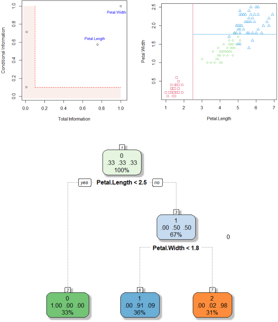
## Multi-Panel Analysis: Information Plots and Decision Tree ### Overview The image presents a multi-panel figure comprising two scatter plots and a decision tree. The top-left plot shows "Conditional Information" vs. "Total Information" with two labeled data points. The top-right plot displays "Petal.Width" vs. "Petal.Length" with data points distinguished by shape. The bottom panel shows a decision tree based on "Petal.Length" and "Petal.Width". ### Components/Axes **Top-Left Plot:** * **X-axis:** Total Information, ranging from 0.0 to 1.0 in increments of 0.2. * **Y-axis:** Conditional Information, ranging from 0.0 to 1.0 in increments of 0.2. * **Data Points:** Two data points are labeled "Petal.Length" and "Petal.Width". * **Highlighted Region:** A rectangular region in the bottom-left corner is highlighted in light red. The region spans from approximately x=0 to x=0.2 and y=0 to y=0.1. **Top-Right Plot:** * **X-axis:** Petal.Length, ranging from 1 to 7 in increments of 1. * **Y-axis:** Petal.Width, ranging from 0.5 to 2.5 in increments of 0.5. * **Data Points:** Three distinct groups of data points, each represented by a different shape: squares, circles, and triangles. * **Decision Boundaries:** A vertical red line at approximately Petal.Length = 2.75 and a horizontal blue line at approximately Petal.Width = 1.8. **Decision Tree:** * **Root Node:** Labeled "1", contains the values "0", ".33 .33 .33", and "100%". The decision rule is "Petal.Length < 2.5". * **Left Child Node:** Labeled "2", contains the values "0", "1.00 .00 .00", and "33%". * **Right Child Node:** Labeled "3", contains the values "1", ".00 .50 .50", and "67%". The decision rule is "Petal.Width < 1.8". * **Left Grandchild Node:** Labeled "6", contains the values "1", ".00 .91 .09", and "36%". * **Right Grandchild Node:** Labeled "7", contains the values "2", ".00 .02 .98", and "31%". ### Detailed Analysis **Top-Left Plot:** * The "Petal.Length" data point is located at approximately (0.75, 0.55). * The "Petal.Width" data point is located at approximately (0.9, 0.95). * Two additional unlabeled data points are present at approximately (0.02, 0.1) and (0.02, 0.7). **Top-Right Plot:** * Squares (likely representing one class) are clustered in the bottom-left corner, with Petal.Length ranging from 1 to 2.5 and Petal.Width ranging from 0.2 to 0.6. * Circles (likely representing another class) are clustered in the middle, with Petal.Length ranging from 3 to 5 and Petal.Width ranging from 1.0 to 1.8. * Triangles (likely representing a third class) are clustered in the top-right corner, with Petal.Length ranging from 4.5 to 7 and Petal.Width ranging from 1.4 to 2.5. **Decision Tree:** * The root node splits the data based on "Petal.Length < 2.5". * The right child node further splits the data based on "Petal.Width < 1.8". * The values within each node likely represent class distributions and percentages. ### Key Observations * The top-left plot seems to represent some information gain or feature importance metric for Petal Length and Petal Width. * The top-right plot shows a clear separation of three classes based on Petal.Length and Petal.Width. * The decision tree attempts to classify the data based on these two features. ### Interpretation The image illustrates a classification problem, likely involving different species of Iris flowers, where the goal is to predict the species based on Petal.Length and Petal.Width. The scatter plot shows that these two features are effective in separating the classes. The decision tree provides a simple rule-based approach to classification, using thresholds on Petal.Length and Petal.Width to assign data points to different classes. The values in the decision tree nodes likely represent the proportion of each class within that node. The highlighted region in the top-left plot might indicate a region of low information or high uncertainty.

## Decision Tree: Iris Dataset Analysis ### Overview The image presents a decision tree visualizing the classification of the Iris dataset based on petal length and petal width. The top portion of the image contains two scatter plots, likely used in the construction or understanding of the decision tree. The bottom portion displays the decision tree itself, with node splits and resulting classifications. ### Components/Axes * **Top-Left Scatter Plot:** * X-axis: Total Information (0.0 to 1.0) * Y-axis: Conditional Information (0.0 to 1.0) * Data Points: Two labeled points: "Petal Length" and "Petal Width". * **Top-Right Scatter Plot:** * X-axis: Petal Length (1.0 to 7.0) * Y-axis: Petal Width (0.0 to 2.5) * Data Points: Three distinct types of markers: circles, squares, and triangles. * **Decision Tree:** * Root Node: "Petal.Length < 2.5" * Second Level Nodes: "Petal.Width < 1.8" (under the "no" branch) * Leaf Nodes: Representing classifications with counts, probabilities, and percentages. * **Legend (within Decision Tree Nodes):** * Number: Total samples at the node. * First Value: Number of samples belonging to class 0. * Second Value: Probability of class 0. * Third Value: Percentage of class 0. ### Detailed Analysis or Content Details **Top-Left Scatter Plot:** The plot shows the relationship between Total Information and Conditional Information for "Petal Length" and "Petal Width". "Petal Length" is located at approximately (0.8, 0.2), while "Petal Width" is at approximately (0.2, 0.8). **Top-Right Scatter Plot:** This plot displays the distribution of petal length versus petal width. * **Circles:** Appear to be concentrated around Petal Length values between 4 and 6, and Petal Width values between 1.0 and 2.5. * **Squares:** Appear to be concentrated around Petal Length values between 1.5 and 3.0, and Petal Width values between 0.5 and 1.5. * **Triangles:** Appear to be concentrated around Petal Length values between 4.5 and 7.0, and Petal Width values between 1.5 and 2.5. **Decision Tree:** * **Root Node (Petal.Length < 2.5):** Contains 7 samples. * "yes" branch leads to a leaf node with 2 samples. * Class 0: 0 samples (0.00, 0.00%) * Class 1: 2 samples (1.00, 100.00%) * Percentage of Class 1: 33% * "no" branch leads to a second-level node (Petal.Width < 1.8). * **Second Level Node (Petal.Width < 1.8):** Contains 5 samples. * "yes" branch leads to a leaf node with 1 sample. * Class 0: 1 sample (0.00, 91.09%) * Class 1: 0 samples (0.00, 9.09%) * Percentage of Class 1: 33% * "no" branch leads to a leaf node with 2 samples. * Class 0: 2 samples (0.02, 98%) * Class 1: 0 samples (0.00, 2%) * Percentage of Class 1: 31% ### Key Observations * The decision tree uses petal length as the primary splitting criterion. * The second split is based on petal width, but only for samples where petal length is greater than or equal to 2.5. * The leaf nodes indicate the classification of the Iris species based on the petal length and width. * The scatter plots suggest a clear separation between the three Iris species based on petal length and width. ### Interpretation The decision tree effectively classifies the Iris dataset based on petal length and width. The tree suggests that petal length is the most important feature for distinguishing between the species, with petal width playing a secondary role. The scatter plots visually confirm the separability of the Iris species based on these two features. The probabilities and percentages in the leaf nodes indicate the confidence of the classification at each node. The tree's structure reflects a hierarchical decision-making process, where the most informative feature is used first to split the data, and subsequent splits refine the classification based on additional features. The data suggests that the Iris species can be accurately classified using a relatively simple decision tree based on petal measurements.

## Scatter Plots and Decision Tree Diagram: Iris Dataset Classification ### Overview The image is a composite technical figure containing three distinct but related visualizations. The top section consists of two scatter plots analyzing feature relationships from what appears to be the Iris flower dataset. The bottom section displays a decision tree classifier trained on the same data. The visualizations collectively demonstrate feature importance, data distribution, and the resulting classification logic. ### Components/Axes **Top-Left Plot: Feature Information Scatter** * **Chart Type:** Scatter plot with annotation. * **X-Axis:** Label: "Total Information". Scale: 0.0 to 1.0, with major ticks at 0.0, 0.2, 0.4, 0.6, 0.8, 1.0. * **Y-Axis:** Label: "Conditional Information". Scale: 0.0 to 1.0, with major ticks at 0.0, 0.2, 0.4, 0.6, 0.8, 1.0. * **Data Points:** Two labeled points. * "Petal.Width": Positioned at approximately (Total Information: 1.0, Conditional Information: 1.0). * "Petal.Length": Positioned at approximately (Total Information: 0.75, Conditional Information: 0.6). * **Other Elements:** A red dashed line forms an L-shape, originating near (0.0, 0.1), extending horizontally to (1.0, 0.1), and vertically to (0.0, 1.0). The area to the left and below this line is shaded in a light pink/beige color. **Top-Right Plot: Petal Dimensions Scatter** * **Chart Type:** Scatter plot with cluster separation lines. * **X-Axis:** Label: "Petal.Length". Scale: 1 to 7, with major ticks at 1, 2, 3, 4, 5, 6, 7. * **Y-Axis:** Label: "Petal.Width". Scale: 0.5 to 2.5, with major ticks at 0.5, 1.0, 1.5, 2.0, 2.5. * **Data Series & Legend (Implied by shape/color):** * **Red Squares:** Clustered in the bottom-left region. X-range: ~1.0 to 2.0. Y-range: ~0.1 to 0.6. * **Green Circles:** Clustered in the central region. X-range: ~3.0 to 5.2. Y-range: ~1.0 to 1.8. * **Blue Triangles:** Clustered in the top-right region. X-range: ~4.5 to 7.0. Y-range: ~1.4 to 2.5. * **Separation Lines:** * **Vertical Red Line:** Positioned at `Petal.Length = 2.5`. * **Horizontal Blue Line:** Positioned at `Petal.Width = 1.8`. **Bottom Diagram: Decision Tree Classifier** * **Chart Type:** Decision tree flow diagram. * **Root Node (Top):** * Box Color: Light green. * Text: `1` (top-right corner), `0` (center), `.33 .33 .33` (middle row), `100%` (bottom). * **First Split Condition:** Text: `Petal.Length < 2.5`. Branches labeled `yes` (left) and `no` (right). * **Left Leaf Node (from "yes"):** * Box Color: Dark green. * Text: `2` (top-right corner), `0` (center), `1.00 .00 .00` (middle row), `33%` (bottom). * **Right Internal Node (from "no"):** * Box Color: Light blue. * Text: `3` (top-right corner), `1` (center), `.00 .50 .50` (middle row), `67%` (bottom). * **Second Split Condition:** Text: `Petal.Width < 1.8`. Branches implied (left for yes, right for no). * **Left Leaf Node (from second split "yes"):** * Box Color: Medium blue. * Text: `6` (top-right corner), `1` (center), `.00 .91 .09` (middle row), `36%` (bottom). * **Right Leaf Node (from second split "no"):** * Box Color: Orange. * Text: `7` (top-right corner), `2` (center), `.00 .02 .98` (middle row), `31%` (bottom). * **Other Text:** A standalone `0` appears to the right of the right internal node. ### Detailed Analysis **Top-Left Plot Analysis:** This plot maps two features, "Petal.Width" and "Petal.Length," on axes of "Total Information" and "Conditional Information." "Petal.Width" scores maximally (1.0) on both metrics, suggesting it is the most informative feature both independently and in context. "Petal.Length" scores lower on both (~0.75, ~0.6). The red dashed line and shaded region likely demarcate a threshold or region of low information value. **Top-Right Plot Analysis:** This plot shows the direct relationship between the two key features. Three distinct clusters are visible, corresponding to the three Iris species (setosa, versicolor, virginica). 1. **Red Square Cluster (Setosa):** Low Petal.Length (1-2) and low Petal.Width (0.1-0.6). Clearly separated from others. 2. **Green Circle Cluster (Versicolor):** Medium Petal.Length (3-5.2) and medium Petal.Width (1.0-1.8). 3. **Blue Triangle Cluster (Virginica):** High Petal.Length (4.5-7.0) and high Petal.Width (1.4-2.5). Some overlap with the versicolor cluster in the Petal.Length dimension, but separation is clearer in the Petal.Width dimension. The vertical red line at `Petal.Length = 2.5` perfectly isolates the red square cluster. The horizontal blue line at `Petal.Width = 1.8` primarily separates the blue triangle cluster from the green circle cluster. **Decision Tree Analysis:** The tree formalizes the splits observed in the scatter plot. 1. **Root Node:** Contains 100% of data, evenly split among three classes (`.33 .33 .33`). 2. **First Split (`Petal.Length < 2.5`):** * **Yes (33% of data):** All samples go to a pure leaf node (class `0`, probability `1.00`). This corresponds to the red square cluster. * **No (67% of data):** Samples go to an internal node with a 50/50 split between classes `1` and `2`. 3. **Second Split (`Petal.Width < 1.8`):** * **Yes (36% of total data):** Leads to a leaf node predominantly class `1` (probability `.91`). This corresponds to the green circle cluster. * **No (31% of total data):** Leads to a leaf node predominantly class `2` (probability `.98`). This corresponds to the blue triangle cluster. ### Key Observations 1. **Perfect Initial Separation:** The feature `Petal.Length` at threshold 2.5 provides a clean, linear separation for one class (setosa, class `0`), accounting for 33% of the dataset. 2. **Feature Hierarchy:** The decision tree confirms the top-left plot's assessment: `Petal.Length` is the most important first split, but `Petal.Width` is crucial for resolving the remaining ambiguity between the other two classes. 3. **Cluster Alignment:** The spatial clusters in the scatter plot map directly to the terminal nodes of the decision tree. The separation lines in the scatter plot (`x=2.5`, `y=1.8`) are the exact splitting criteria used by the tree. 4. **Data Distribution:** The dataset is perfectly balanced (33% per class at the root). The final leaf nodes contain 33%, 36%, and 31% of the data, respectively, showing a very balanced final classification. ### Interpretation This composite figure is a classic example of **exploratory data analysis (EDA) followed by model interpretation** for a classification task on the Iris dataset. * **What the data suggests:** The physical measurements of Iris petals contain highly discriminative information. There exists a species (setosa) with distinctly small petals, making it trivially identifiable. The other two species (versicolor and virginica) have overlapping petal lengths but are separable by petal width, suggesting a morphological distinction where virginica flowers are not just longer but also wider. * **How elements relate:** The top-left plot provides a meta-analysis of feature utility. The top-right plot visualizes the raw data and the proposed decision boundaries. The bottom diagram shows the algorithmic implementation of those boundaries. The red and blue lines in the scatter plot are not arbitrary; they are the visual manifestations of the logic encoded in the tree nodes. * **Notable patterns/anomalies:** The perfect initial split is a hallmark of the Iris dataset and indicates a very strong, simple feature. The slight overlap between green and blue clusters in the scatter plot explains why the second split is not 100% pure (91% and 98% probabilities). The model achieves high accuracy with a very simple, interpretable structure of just two rules. The "Total Information" plot suggests that while `Petal.Length` is a strong first splitter, `Petal.Width` holds more comprehensive information when considered alone.

## Scatter Plots and Decision Tree: Iris Petal Measurements and Classification ### Overview The image contains two scatter plots and a decision tree. The left scatter plot visualizes "Total Information" vs. "Conditional Information" with labeled data points. The right scatter plot shows "Petal Length" vs. "Petal Width" with color-coded shapes. The decision tree below classifies data based on petal measurements, with node values and split conditions. --- ### Components/Axes #### Left Scatter Plot - **X-axis**: Total Information (0.0–1.0) - **Y-axis**: Conditional Information (0.0–1.0) - **Data Points**: - (0.1, 0.7): Labeled "Petal Width" - (0.8, 0.6): Labeled "Petal Length" - (0.9, 0.9): Labeled "Petal Width" - **Shaded Area**: Light pink rectangle spanning (0,0) to (1,0.5) - **Dashed Line**: Red dashed line at y=0.5 (Conditional Information threshold) #### Right Scatter Plot - **X-axis**: Petal Length (1–7) - **Y-axis**: Petal Width (0–2.5) - **Data Points**: - **Red Squares**: Clustered near (1–2, 0–1) - **Blue Triangles**: Spread across (4–7, 1.5–2.5) - **Green Circles**: Distributed between (3–5, 0.5–1.5) - **Dashed Lines**: - Vertical red line at x=3 (Petal Length threshold) - Horizontal blue line at y=1.5 (Petal Width threshold) - **Legend**: Top-right, associating colors with shapes (red=squares, blue=triangles, green=circles) #### Decision Tree - **Root Node (1)**: - Condition: `Petal.Length < 2.5` - Yes → Node 2 (green) - No → Node 3 (blue) - **Node 2**: - Values: `[0, 33, 33, 33]` - Percentage: 100% - **Node 3**: - Condition: `Petal.Width < 1.8` - Yes → Node 6 (blue) - No → Node 7 (orange) - **Leaf Nodes**: - Node 6: `[1, 0.00, 0.91, 0.09]`, 36% - Node 7: `[2, 0.00, 0.02, 0.98]`, 31% --- ### Detailed Analysis #### Left Scatter Plot - **Trends**: - Petal Width (0.1, 0.7) and Petal Length (0.8, 0.6) show high conditional information. - Petal Width (0.9, 0.9) lies near the upper-right corner, suggesting maximum conditional information. - **Shaded Area**: Indicates a region where conditional information is ≤0.5. Only Petal Length (0.8, 0.6) partially overlaps this area. #### Right Scatter Plot - **Trends**: - **Red Squares**: Low petal length (1–2) and width (0–1), likely representing a specific class (e.g., Setosa). - **Blue Triangles**: High petal length (4–7) and width (1.5–2.5), possibly Virginica. - **Green Circles**: Intermediate values (3–5, 0.5–1.5), likely Versicolor. - **Dashed Lines**: Thresholds at Petal Length=3 and Width=1.5 align with class separations. #### Decision Tree - **Splits**: - Root splits on `Petal.Length < 2.5` (100% accuracy for Node 2). - Node 3 splits on `Petal.Width < 1.8`, with 67% accuracy for Node 6 and 31% for Node 7. - **Node Values**: - Node 2: All values = 33 (100% confidence in a single class). - Node 6: 1 instance of class 0, 91% class 1, 9% class 2. - Node 7: 2 instances of class 0, 2% class 1, 98% class 2. --- ### Key Observations 1. **Feature Importance**: Petal Width has higher conditional information than Petal Length in the left plot. 2. **Class Separation**: The right plot shows distinct clusters for red squares (low length/width), blue triangles (high length/width), and green circles (intermediate). 3. **Decision Tree Logic**: - Petal Length < 2.5 perfectly separates one class (Node 2). - Petal Width < 1.8 further splits remaining data, with higher accuracy for shorter widths (Node 6). --- ### Interpretation - **Data Relationships**: - The left plot quantifies feature importance, showing Petal Width as more informative. - The right plot visualizes class distributions, with clear separations along petal length and width. - **Model Behavior**: - The decision tree prioritizes Petal Length first, then Petal Width, reflecting their importance. - Node 2’s 100% accuracy suggests a strong class boundary at Petal.Length < 2.5. - **Anomalies**: - Petal Width (0.9, 0.9) in the left plot has the highest conditional information, indicating it may be a critical feature for distinguishing classes. - Node 7’s low accuracy (31%) suggests uncertainty in classifying samples with Petal.Length ≥2.5 and Width ≥1.8. This analysis demonstrates how petal measurements correlate with classification confidence and how the decision tree leverages these features for prediction.