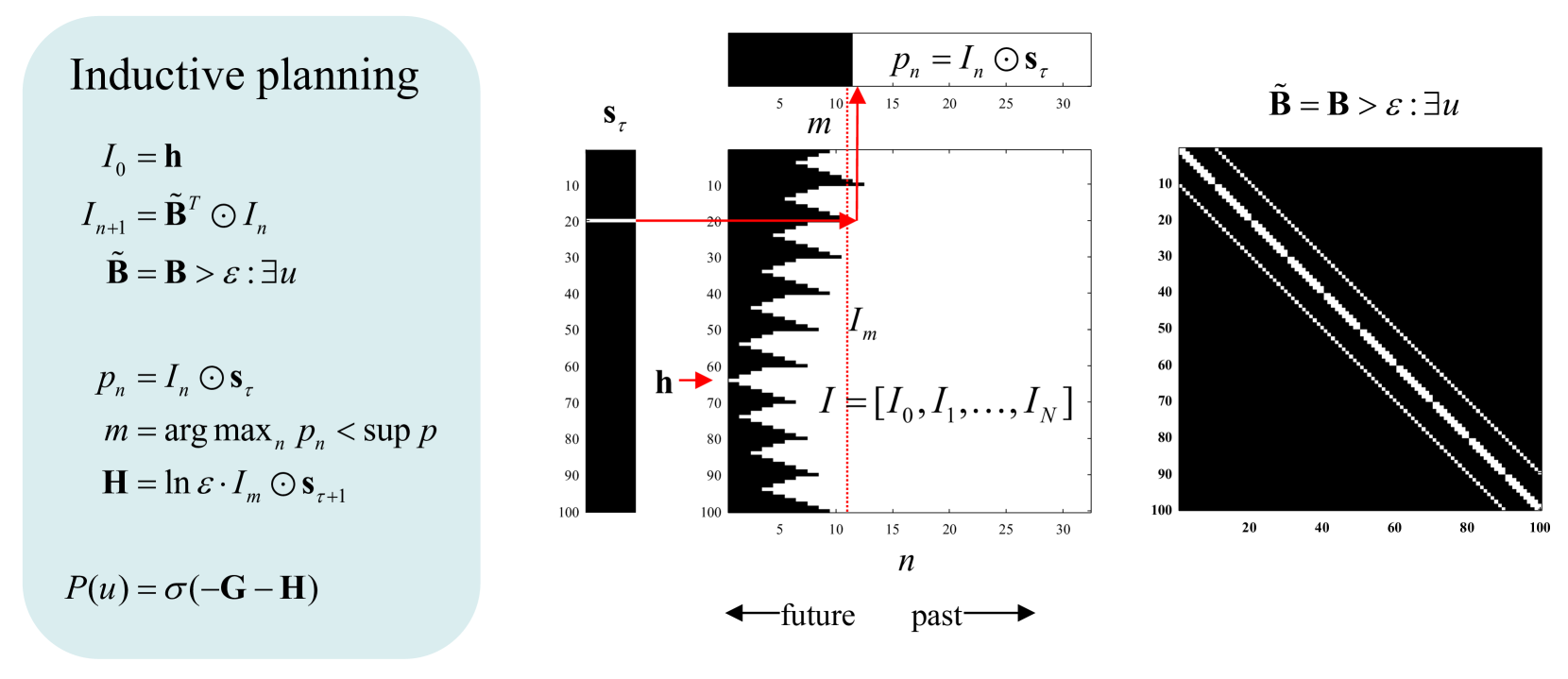
## Technical Diagram: Inductive Planning Process ### Overview The image is a composite technical diagram illustrating a mathematical framework for "Inductive planning." It consists of three interconnected panels: a left panel containing a set of equations, a central panel visualizing a sequence of states and their relationships, and a right panel displaying a specific matrix structure. Red arrows are used to link conceptual elements across the panels. ### Components/Axes **Left Panel (Equations):** * **Title:** "Inductive planning" * **Equations (transcribed precisely):** 1. `I₀ = h` 2. `Iₙ₊₁ = B̃ᵀ ⊙ Iₙ` 3. `B̃ = B > ε : ∃u` 4. `pₙ = Iₙ ⊙ s_τ` 5. `m = arg maxₙ pₙ < sup p` 6. `H = ln ε · Iₘ ⊙ s_{τ+1}` 7. `P(u) = σ(-G - H)` **Central Panel (State Sequence Visualization):** * **Axes:** * Horizontal axis (bottom): Labeled `n`, with tick marks at 5, 10, 15, 20, 25, 30. An arrow below points left with the label `←future` and right with the label `past→`. * Vertical axis (left): Labeled `m`, with tick marks from 10 to 100 in increments of 10. * **Key Elements:** * A vertical black bar on the far left labeled `s_τ`. * A large central matrix labeled `I = [I₀, I₁, ..., I_N]`. This matrix is primarily black with a white, jagged, horizontal pattern running through it. * A horizontal red arrow originates from the `s_τ` bar at approximately `m=20` and points right into the `I` matrix. * A vertical red dashed line runs through the `I` matrix at approximately `n=12`. It is labeled `Iₘ`. * A horizontal red arrow originates from the top of the `Iₘ` line and points upward to a small horizontal bar chart. * A small horizontal bar chart at the top is labeled `pₙ = Iₙ ⊙ s_τ`. Its horizontal axis has tick marks from 5 to 30. * A label `h` with a red arrow points to the `I` matrix at approximately `m=65, n=0`. **Right Panel (Matrix Plot):** * **Title/Label:** `B̃ = B > ε : ∃u` * **Axes:** * Horizontal axis (bottom): Tick marks at 20, 40, 60, 80, 100. * Vertical axis (left): Tick marks at 10, 20, 30, 40, 50, 60, 70, 80, 90, 100. * **Content:** A square, black-and-white matrix plot. It shows a strong white diagonal line from the top-left to bottom-right corner, accompanied by several parallel, fainter white lines offset from the main diagonal. ### Detailed Analysis The diagram visually maps the mathematical operations defined in the left panel onto the structures in the central and right panels. 1. **Equation Flow:** The process begins with an initial state `I₀ = h`. The state is iteratively updated via `Iₙ₊₁ = B̃ᵀ ⊙ Iₙ`, where `B̃` is a thresholded version of a matrix `B` (defined as `B̃ = B > ε : ∃u`). The right panel visualizes this `B̃` matrix, showing a banded diagonal structure. 2. **State Evaluation:** At each step `n`, a value `pₙ` is computed as the dot product (`⊙`) of the current state `Iₙ` and a target or sensory vector `s_τ`. The top bar chart in the central panel visualizes these `pₙ` values across `n`. 3. **State Selection:** The index `m` is selected as the argument maximizing `pₙ`, subject to the constraint that `pₙ` is less than the supremum of `p` (`m = arg maxₙ pₙ < sup p`). This selected state `Iₘ` is highlighted by the vertical red dashed line in the central matrix `I`. 4. **Heuristic Computation:** A heuristic `H` is computed using the selected state `Iₘ` and the *next* sensory input `s_{τ+1}`: `H = ln ε · Iₘ ⊙ s_{τ+1}`. 5. **Policy Output:** Finally, a policy or probability `P(u)` is generated by passing the negative sum of two terms (`G` and `H`) through a sigmoid function `σ`: `P(u) = σ(-G - H)`. ### Key Observations * **Spatial Linking:** The red arrows create a clear visual narrative: the sensory input `s_τ` influences the state matrix `I`; a specific state `Iₘ` is selected based on the computed `pₙ` values; this selection then feeds into the calculation of `H`. * **Matrix Structure:** The `B̃` matrix in the right panel is not random. Its strong diagonal and parallel off-diagonals suggest a structured, possibly time-lagged or spatially-localized, transition or influence matrix. * **State Matrix Texture:** The central `I` matrix is not uniform. The white, jagged horizontal pattern indicates that the state representation is sparse or has a specific, non-random structure across the `m` dimension for each time step `n`. * **Temporal Direction:** The axis labels `←future` and `past→` indicate that increasing `n` corresponds to moving backward in time (toward the past), which is a common convention in some planning or sequence modeling contexts. ### Interpretation This diagram outlines a computational framework for inductive planning, likely in an AI or cognitive modeling context. The process involves: 1. **Maintaining a Belief State (`I`):** A structured internal representation (`I`) is updated over time (`n`) based on a transition model (`B̃`). 2. **Evaluating Against Goals:** The current belief state is continuously evaluated (`pₙ`) against a target or sensory goal (`s_τ`). 3. **Selecting a Reference Point:** A specific past state (`Iₘ`) that best matched the goal (but was not a perfect match, due to the `< sup p` constraint) is selected. This acts as an inductive reference point. 4. **Generating a Heuristic:** Using this reference state and *new* sensory information (`s_{τ+1}`), a heuristic `H` is computed. This heuristic likely guides future planning or action selection. 5. **Producing a Policy:** The final output is a policy `P(u)`, which is a function of this learned heuristic `H` and another term `G` (not defined in the diagram, possibly a cost or prior). The core idea appears to be using past experiences (stored in `I` and selected via `Iₘ`) to inductively generate heuristics for decision-making in new, but related, situations. The structured nature of `B̃` and `I` suggests the model exploits specific temporal or spatial regularities in the problem domain.