## Scaling Laws Comparison: Validation Loss and N/D Ratio vs. Compute (FLOPs)
### Overview
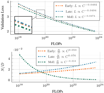
The image contains two vertically stacked line charts sharing a common x-axis. Both charts plot different metrics against computational cost (FLOPs) on a logarithmic scale, comparing three distinct model scaling strategies: "Early," "Late," and "MoE" (Mixture of Experts). The charts illustrate scaling laws, showing how performance and architectural ratios change with increased compute.
### Components/Axes
**Common X-Axis (Both Charts):**
* **Label:** `FLOPs`
* **Scale:** Logarithmic (base 10).
* **Range:** Approximately `10^18` to `10^24`.
* **Major Ticks:** `10^18`, `10^20`, `10^22`, `10^24`.
**Top Chart:**
* **Y-Axis Label:** `Validation Loss`
* **Y-Axis Scale:** Linear.
* **Y-Axis Range:** Approximately 2 to 4.
* **Legend (Top-Right Corner):**
* Orange dashed line: `Early: L ∝ C^(-0.0492)`
* Blue dashed line: `Late: L ∝ C^(-0.0494)`
* Green dashed line: `MoE: L ∝ C^(-0.0474)`
* **Inset:** A zoomed-in view of the region between approximately `10^18` and `10^19` FLOPs is shown in a box in the top-left quadrant of the chart area.
**Bottom Chart:**
* **Y-Axis Label:** `N/D` (with a multiplier `·10^-2` at the top of the axis, indicating values are scaled by 0.01).
* **Y-Axis Scale:** Linear.
* **Y-Axis Range:** 0 to 4 (representing 0 to 0.04 after applying the `10^-2` multiplier).
* **Legend (Top-Right Corner):**
* Orange dashed line: `Early: N/D ∝ C^(0.053)`
* Blue dashed line: `Late: N/D ∝ C^(0.076)`
* Green dashed line: `MoE: N/D ∝ C^(-0.312)`
### Detailed Analysis
**Top Chart (Validation Loss vs. FLOPs):**
* **Trend Verification:** All three lines slope downward from left to right, indicating that Validation Loss decreases as computational cost (FLOPs) increases.
* **Data Series & Scaling Laws:**
1. **Early (Orange):** Follows the power law `L ∝ C^(-0.0492)`. The line starts highest at low FLOPs and decreases steadily.
2. **Late (Blue):** Follows the power law `L ∝ C^(-0.0494)`. This line is nearly parallel to and slightly below the "Early" line across the entire range.
3. **MoE (Green):** Follows the power law `L ∝ C^(-0.0474)`. This line starts the lowest at `10^18` FLOPs but has the shallowest slope (least negative exponent). It intersects and rises above the "Late" line at approximately `10^20` FLOPs and appears to cross above the "Early" line at a higher FLOP count (estimated ~`10^22` FLOPs).
* **Inset Detail:** The inset confirms the initial ordering at low compute: MoE (lowest loss) < Late < Early (highest loss).
**Bottom Chart (N/D vs. FLOPs):**
* **Trend Verification:**
* The "Early" (Orange) and "Late" (Blue) lines slope upward.
* The "MoE" (Green) line slopes sharply downward.
* **Data Series & Scaling Laws:**
1. **Early (Orange):** Follows `N/D ∝ C^(0.053)`. It shows a gradual, steady increase from ~1.2 (0.012) at `10^18` FLOPs to ~2.2 (0.022) at `10^24` FLOPs.
2. **Late (Blue):** Follows `N/D ∝ C^(0.076)`. It increases more steeply than "Early," starting near 1.0 (0.010) and ending near 3.5 (0.035).
3. **MoE (Green):** Follows `N/D ∝ C^(-0.312)`. It starts highest at ~4.8 (0.048) at `10^18` FLOPs and decreases rapidly, approaching 0 near `10^24` FLOPs.
* **Crossover Points:** The "MoE" line crosses below the "Early" line at approximately `10^19` FLOPs and below the "Late" line shortly after.
### Key Observations
1. **Inverse Relationship in Top Chart:** All strategies show diminishing returns (decreasing loss) with more compute, but the rate of improvement (exponent magnitude) is very similar for Early and Late scaling, and slightly worse for MoE.
2. **Divergent Architectural Trends:** The bottom chart reveals a fundamental difference. For standard "Early" and "Late" scaling, the ratio `N/D` (likely representing a parameter count ratio, e.g., Numel/Depth) *increases* with compute. For "MoE" scaling, this ratio *decreases* sharply.
3. **MoE Crossover:** The MoE strategy is most effective (lowest loss) at lower compute budgets (`<10^20` FLOPs) but becomes less effective than the other strategies at very high compute, as indicated by its shallower loss curve slope.
4. **Precision of Laws:** The scaling exponents are provided to four decimal places, suggesting they are derived from precise fits to empirical data.
### Interpretation
This visualization compares the efficiency and architectural consequences of different neural network scaling paradigms.
* **What the data suggests:** The "Early" and "Late" scaling methods (likely referring to when capacity is increased during training or in which parts of the model) follow very similar, predictable power-law improvements in loss. Their architectural ratio (`N/D`) grows with compute, suggesting they become relatively wider or shallower. In contrast, the "MoE" strategy trades off a different scaling trajectory. It achieves better loss at low compute but scales less efficiently. Crucially, its architecture evolves in the opposite direction—`N/D` shrinks, meaning it likely becomes relatively deeper or narrower as it scales.
* **How elements relate:** The two charts are linked. The top chart shows the *performance outcome* (loss) of each scaling law. The bottom chart shows a key *architectural driver* (the `N/D` ratio) that changes as a consequence of following that law. The crossover in the top chart is explained by the diverging trends in the bottom chart.
* **Notable implications:** The data argues that MoE models have a distinct and less favorable scaling law for loss (`C^(-0.0474)` vs. ~`C^(-0.0493)`). Their architectural advantage (high `N/D` at low compute) diminishes rapidly. For projects with massive compute budgets (`>10^22` FLOPs), traditional "Late" scaling appears to offer the best loss. The choice of scaling strategy is therefore highly dependent on the available computational budget.