## Network Diagram: Adaptor Architectures
### Overview
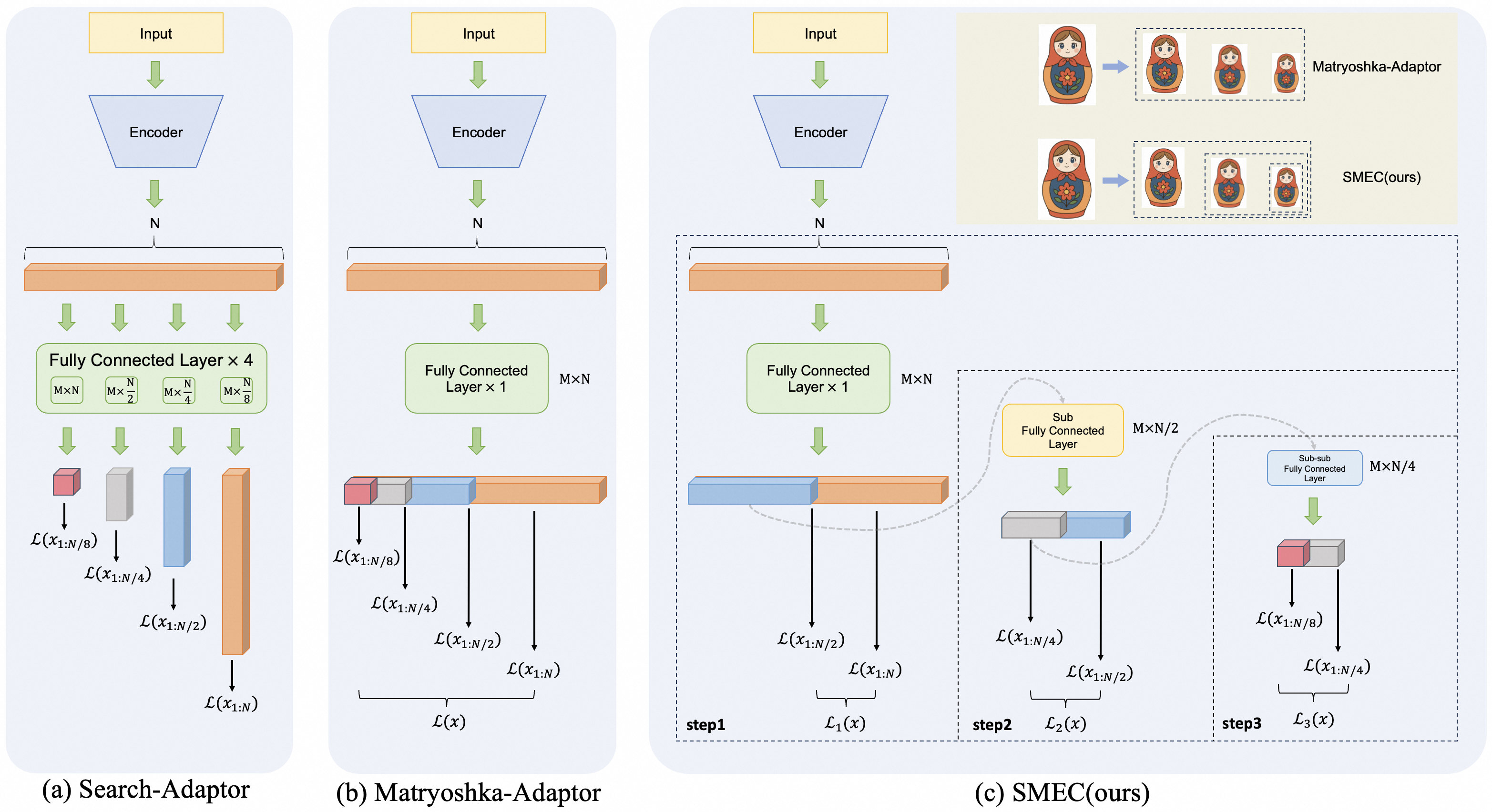
The image presents three different adaptor architectures for neural networks: Search-Adaptor, Matryoshka-Adaptor, and SMEC(ours). Each architecture illustrates how input data flows through an encoder and subsequent layers, with variations in the structure and dimensionality of these layers.
### Components/Axes
* **Input:** Yellow rectangle at the top of each architecture, labeled "Input".
* **Encoder:** Blue trapezoid below the input, labeled "Encoder".
* **N:** Indicates the output of the encoder.
* **Fully Connected Layers:** Green rectangles representing fully connected layers with varying dimensions.
* **Sub Fully Connected Layer:** Yellow rectangle representing a sub fully connected layer.
* **Sub-sub Fully Connected Layer:** Blue rectangle representing a sub-sub fully connected layer.
* **Data Flow:** Green arrows indicate the direction of data flow.
* **Output Layers:** Represented by stacked blocks of different colors (red, gray, blue, orange) with corresponding labels L(x1:N/8), L(x1:N/4), L(x1:N/2), and L(x1:N).
* **Matryoshka Doll Analogy:** Top-right corner shows Matryoshka dolls to illustrate the concept of nested structures in Matryoshka-Adaptor and SMEC.
### Detailed Analysis
#### (a) Search-Adaptor
* **Input** flows into the **Encoder**, producing an output of size **N**.
* This output is fed into a **Fully Connected Layer x 4**. This layer is split into four sub-layers with dimensions: MxN, Mx(N/2), Mx(N/4), and Mx(N/8).
* The outputs of these sub-layers are then processed individually, resulting in output layers labeled as follows:
* Red block: L(x1:N/8)
* Gray block: L(x1:N/4)
* Blue block: L(x1:N/2)
* Orange block: L(x1:N)
#### (b) Matryoshka-Adaptor
* **Input** flows into the **Encoder**, producing an output of size **N**.
* This output is fed into a **Fully Connected Layer x 1** with dimensions MxN.
* The output is then split and processed, resulting in output layers labeled as follows:
* Red block: L(x1:N/8)
* Gray block: L(x1:N/4)
* Blue block: L(x1:N/2)
* Orange block: L(x1:N)
* The combined output is labeled L(x).
#### (c) SMEC(ours)
* **Input** flows into the **Encoder**, producing an output of size **N**.
* This output is fed into a **Fully Connected Layer x 1** with dimensions MxN (Step 1).
* The output is then split and processed, resulting in output layers labeled as follows:
* Blue block: L(x1:N/2)
* Orange block: L(x1:N)
* The combined output is labeled L1(x).
* A **Sub Fully Connected Layer** with dimensions MxN/2 is applied (Step 2).
* The output is then split and processed, resulting in output layers labeled as follows:
* Gray block: L(x1:N/4)
* Blue block: L(x1:N/2)
* The combined output is labeled L2(x).
* A **Sub-sub Fully Connected Layer** with dimensions MxN/4 is applied (Step 3).
* The output is then split and processed, resulting in output layers labeled as follows:
* Red block: L(x1:N/8)
* Gray block: L(x1:N/4)
* The combined output is labeled L3(x).
* The top-right corner shows Matryoshka dolls to illustrate the concept of nested structures in SMEC.
### Key Observations
* The Search-Adaptor uses parallel fully connected layers, while Matryoshka-Adaptor and SMEC use a single fully connected layer with sequential processing.
* SMEC(ours) introduces sub-layers to further refine the output.
* The Matryoshka doll analogy visually represents the nested structure of the Matryoshka-Adaptor and SMEC architectures.
### Interpretation
The diagrams illustrate different approaches to adapting neural networks. The Search-Adaptor explores multiple parallel pathways, while the Matryoshka-Adaptor and SMEC architectures focus on hierarchical processing. SMEC(ours) appears to be a more refined version of the Matryoshka-Adaptor, incorporating multiple sub-layers to achieve a more granular output. The Matryoshka doll analogy emphasizes the recursive and nested nature of these architectures, suggesting a design that progressively refines the input data.