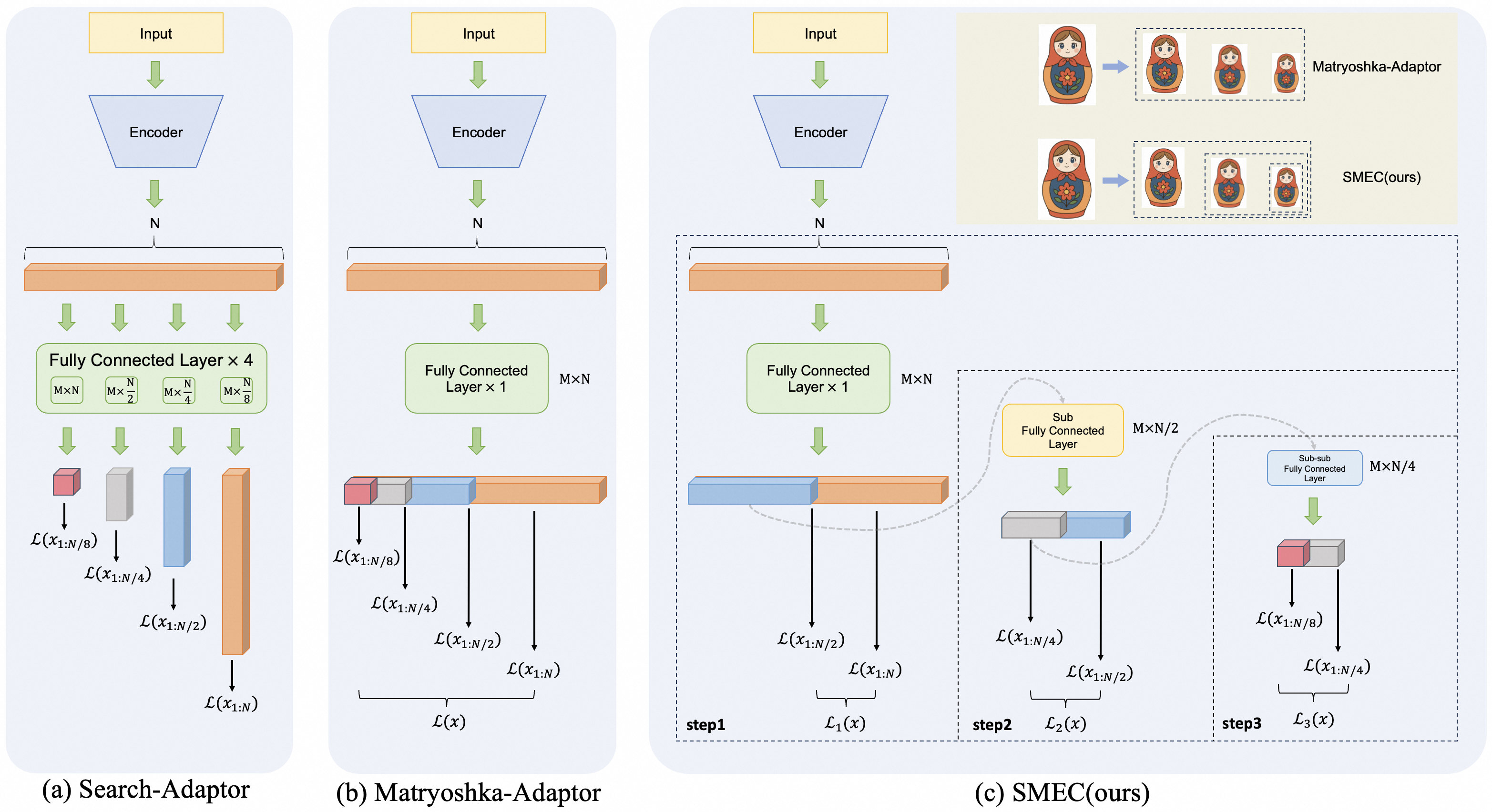
\n ## Technical Diagram: Comparison of Three Adaptor Architectures ### Overview The image presents a side-by-side comparison of three neural network adaptor architectures, labeled (a) Search-Adaptor, (b) Matryoshka-Adaptor, and (c) SMEC(ours). Each diagram illustrates the flow of data from an input through an encoder and subsequent fully connected layers, culminating in various loss function calculations. The diagrams use a consistent visual language: yellow boxes for input, blue trapezoids for encoders, orange bars for feature vectors, green boxes for fully connected layers, and colored blocks (red, grey, blue, orange) to represent different dimensional outputs. The rightmost diagram (c) includes an inset analogy using Matryoshka dolls to conceptualize the method. ### Components/Axes **Common Components Across All Diagrams:** * **Input:** A yellow rectangular box at the top. * **Encoder:** A blue trapezoidal block below the input. * **N:** A label indicating the dimension of the feature vector output by the encoder. * **Feature Vector:** An orange horizontal bar representing the encoded output of dimension N. * **Loss Functions:** Denoted by the script L, e.g., `L(x_{1:N})`. These are the final outputs of each branch. **Diagram-Specific Components:** **(a) Search-Adaptor:** * **Layer Label:** "Fully Connected Layer × 4" inside a green box. * **Sub-layer Dimensions:** Four smaller green boxes below, labeled: `M×N`, `M×N/2`, `M×N/4`, `M×N/8`. * **Output Blocks:** Four vertical colored blocks (red, grey, blue, orange) of decreasing height, each feeding into a separate loss function. * **Loss Functions:** Four distinct losses: `L(x_{1:N/8})`, `L(x_{1:N/4})`, `L(x_{1:N/2})`, `L(x_{1:N})`. **(b) Matryoshka-Adaptor:** * **Layer Label:** "Fully Connected Layer × 1" inside a green box, with `M×N` noted to its right. * **Output Structure:** A single, segmented horizontal bar composed of four contiguous colored blocks (red, grey, blue, orange). * **Loss Functions:** Four losses are calculated from prefixes of the segmented bar: `L(x_{1:N/8})`, `L(x_{1:N/4})`, `L(x_{1:N/2})`, `L(x_{1:N})`. These are collectively bracketed as `L(x)`. **(c) SMEC(ours):** * **Inset Analogy (Top-Right):** A beige box containing two rows. * **Row 1:** Labeled "Matryoshka-Adaptor". Shows a large Matryoshka doll pointing to three smaller, nested dolls. * **Row 2:** Labeled "SMEC(ours)". Shows a large Matryoshka doll pointing to three separate, non-nested dolls of different sizes. * **Main Architecture:** A three-step process enclosed in a dashed box. * **Step 1 (step1):** A green box "Fully Connected Layer × 1" (`M×N`). Outputs a segmented bar (blue, orange) leading to losses `L(x_{1:N/2})` and `L(x_{1:N})`, bracketed as `L₁(x)`. * **Step 2 (step2):** A yellow box "Sub Fully Connected Layer" (`M×N/2`). Takes input from the blue segment of Step 1. Outputs a segmented bar (grey, blue) leading to losses `L(x_{1:N/4})` and `L(x_{1:N/2})`, bracketed as `L₂(x)`. * **Step 3 (step3):** A blue box "Sub-sub Fully Connected Layer" (`M×N/4`). Takes input from the grey segment of Step 2. Outputs a segmented bar (red, grey) leading to losses `L(x_{1:N/8})` and `L(x_{1:N/4})`, bracketed as `L₃(x)`. ### Detailed Analysis **Data Flow and Dimensionality:** 1. **Search-Adaptor (a):** The encoder output (dim N) is fed into four *parallel* fully connected layers of decreasing width (`M×N` to `M×N/8`). Each produces an independent output vector, and a separate loss is computed for each. This suggests a search over multiple representation granularities simultaneously. 2. **Matryoshka-Adaptor (b):** The encoder output (dim N) is processed by a *single* fully connected layer (`M×N`). The resulting vector is conceptually segmented. Losses are computed on progressively longer prefixes of this single vector (from the first `N/8` dimensions to all `N` dimensions). This creates nested, multi-scale representations within one vector. 3. **SMEC(ours) (c):** This is a *sequential, hierarchical* process. * **Step 1:** Processes the full N-dimensional input to produce a coarse, two-segment representation. * **Step 2:** Refines one segment (the blue one, representing the first `N/2` dimensions) using a sub-layer, creating a finer two-segment representation. * **Step 3:** Further refines a sub-segment (the grey one from Step 2, representing the first `N/4` dimensions) using a sub-sub-layer. * Losses are computed at each step on the available segments. The Matryoshka doll analogy highlights that SMEC creates separate, non-nested representations at each scale, unlike the nested dolls of the Matryoshka-Adaptor. ### Key Observations * **Structural Paradigm Shift:** The diagrams show a clear evolution from parallel multi-branch (a), to single-branch nested (b), to hierarchical sequential refinement (c). * **Loss Function Consistency:** All three methods ultimately compute losses for the same four dimensional granularities: `N/8`, `N/4`, `N/2`, and `N`. The difference lies in *how* the representations for these granularities are generated. * **Visual Metaphor:** The Matryoshka doll inset in (c) is a critical explanatory element. It visually argues that the proposed SMEC method avoids the "nesting" constraint of the Matryoshka-Adaptor, potentially allowing for more independent and flexible feature learning at each scale. * **Spatial Grounding:** In diagram (c), the "Sub Fully Connected Layer" (step2) is positioned to the right of and below the main step1 block, with a dashed arrow indicating it processes a segment from step1. Similarly, the "Sub-sub Fully Connected Layer" (step3) is further right and below step2, processing a segment from step2. This spatial arrangement reinforces the sequential, hierarchical nature of the process. ### Interpretation This technical diagram serves as a conceptual blueprint for different methods of creating multi-scale or multi-granularity representations in neural networks, likely for tasks like retrieval or metric learning where representation size impacts efficiency and performance. * **What the data suggests:** The progression from (a) to (c) suggests a research trajectory aimed at improving the efficiency and independence of multi-scale feature learning. Search-Adaptor (a) is computationally expensive (4 parallel layers). Matryoshka-Adaptor (b) is efficient (1 layer) but couples all scales via nesting. SMEC (c) proposes a middle ground: a structured, sequential process that maintains some independence between scales (as per the doll analogy) while potentially being more parameter-efficient than the parallel approach. * **How elements relate:** The core relationship is between the dimensionality of the feature vector (`N`, `N/2`, etc.) and the architectural path taken to produce a useful representation at that scale. The loss functions `L(x_{1:N/k})` are the common objective, but the means of generating `x_{1:N/k}` differ fundamentally. * **Notable anomalies/outliers:** The most significant "outlier" is the SMEC architecture itself. Its three-step, dashed-box structure breaks the visual pattern of the first two diagrams, emphasizing its novel, proposed nature. The explicit use of a cultural metaphor (Matryoshka dolls) to explain a technical concept is also a distinctive communicative choice. * **Underlying purpose:** The diagram is designed to persuade. It visually argues that the authors' method (SMEC) combines the benefits of the prior approaches—multi-scale learning—while introducing a new hierarchical decomposition that may offer advantages in representation independence or training dynamics. The careful labeling of all dimensions (`M×N`, `M×N/2`, etc.) provides the necessary technical rigor to support this conceptual argument.