## Diagram: SVD Split vs. SVD Joint Architectures
### Overview
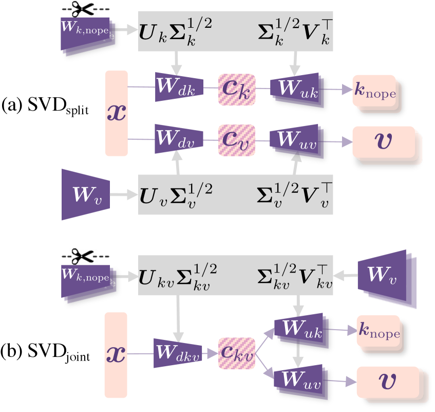
The image compares two Singular Value Decomposition (SVD) architectures for processing input data `x`:
- **(a) SVD_split**: Separates processing paths for `k` (noise) and `v` (signal).
- **(b) SVD_joint**: Combines processing paths for `k` and `v` into a unified framework.
Both architectures use matrix factorization, orthogonal transformations, and noise suppression mechanisms.
---
### Components/Axes
#### Key Elements:
1. **Matrices**:
- `W_k,nope`, `W_v`: Input weight matrices for noise and signal.
- `W_dk`, `W_dv`: Decomposition matrices for `k` and `v`.
- `W_uk`, `W_uv`: Reconstruction matrices for `k` and `v`.
- `C_k`, `C_v`: Cross-covariance matrices (checkerboard patterns).
- `C_kv`: Joint cross-covariance matrix.
2. **Operations**:
- `U_k Σ_k^1/2`, `Σ_v^1/2 V_v^T`: Singular value decomposition (SVD) steps.
- `U_kv Σ_kv^1/2 V_kv^T`: Joint SVD step.
3. **Outputs**:
- `k_nope`: Suppressed noise component.
- `v`: Reconstructed signal component.
4. **Flow**:
- Arrows indicate matrix multiplication and data flow.
- Dashed lines (`W_k,nope`) denote optional or auxiliary components.
---
### Detailed Analysis
#### (a) SVD_split Architecture
1. **Input**:
- `x` is split into `W_dk` (for `k`) and `W_dv` (for `v`).
2. **Processing**:
- `W_dk` → `C_k` → `W_uk` → `k_nope` (noise suppression).
- `W_dv` → `C_v` → `W_uv` → `v` (signal reconstruction).
3. **SVD Steps**:
- `W_v` → `U_v Σ_v^1/2` → `Σ_v^1/2 V_v^T` (orthogonal transformation).
#### (b) SVD_joint Architecture
1. **Input**:
- `x` is processed through `W_dkv` (combined decomposition).
2. **Processing**:
- `W_dkv` → `C_kv` → Branching to `W_uk` (noise) and `W_uv` (signal).
3. **SVD Steps**:
- `W_k,nope` → `U_kv Σ_kv^1/2` → `Σ_kv^1/2 V_kv^T` (joint SVD).
---
### Key Observations
1. **Noise Suppression**:
- Both methods suppress `k_nope` (noise) via orthogonal transformations.
- SVD_joint uses a shared covariance matrix `C_kv`, potentially improving noise correlation handling.
2. **Computational Complexity**:
- SVD_split requires separate SVDs for `k` and `v`, increasing computation.
- SVD_joint combines SVD steps, reducing redundancy.
3. **Signal Reconstruction**:
- `v` is reconstructed via `W_uv` in both methods, but SVD_joint may leverage joint statistics for better accuracy.
---
### Interpretation
- **Technical Implications**:
- SVD_joint likely offers computational efficiency by unifying SVD steps and covariance modeling.
- SVD_split provides modularity, useful for scenarios where noise and signal processing require independent tuning.
- **Practical Use Cases**:
- SVD_joint: Suitable for high-dimensional data with correlated noise/signal.
- SVD_split: Preferred when interpretability or separate noise/signal handling is critical.
- **Uncertainties**:
- The exact impact of `C_kv` on performance depends on data structure (not quantified here).
- Trade-offs between accuracy and computational cost are implied but not explicitly measured.
---
**Note**: No numerical values or explicit legends are present. The diagram focuses on architectural differences rather than empirical results.