TECHNICAL ASSET FINGERPRINT
40125d366cb9011ef31c8130
Click to view fullscreen
Press ESC or click to close
FOUND IN PAPERS
EXPERT: healer-alpha-free VERSION 1
RUNTIME: free/openrouter/healer-alpha
INTEL_VERIFIED
## [Chart Type: Dual Line Charts with Multiple Series]
### Overview
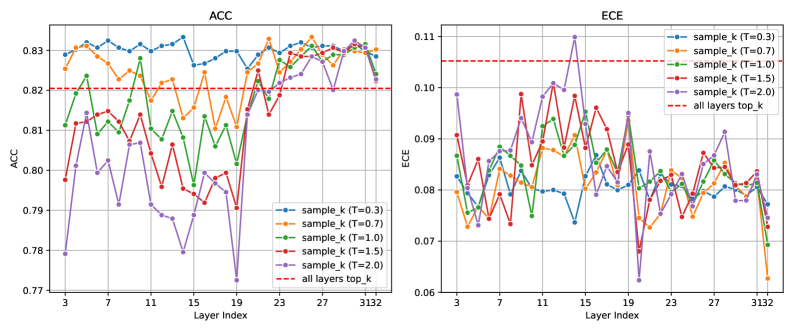
The image displays two side-by-side line charts comparing the performance of a model across different layers, using two metrics: Accuracy (ACC) and Expected Calibration Error (ECE). Each chart plots multiple data series corresponding to different "sample_k" configurations with varying temperature (T) values, alongside a baseline reference line.
### Components/Axes
**Common Elements:**
* **X-Axis (Both Charts):** Labeled "Layer Index". The axis is marked with major ticks at 3, 7, 11, 15, 19, 23, 27, 31, and 32. The scale appears linear.
* **Legend (Bottom-Right of Each Chart):** Contains six entries:
1. `sample_k (T=0.3)`: Blue line with circular markers.
2. `sample_k (T=0.7)`: Orange line with square markers.
3. `sample_k (T=1.0)`: Green line with upward-pointing triangle markers.
4. `sample_k (T=1.5)`: Red line with downward-pointing triangle markers.
5. `sample_k (T=2.0)`: Purple line with diamond markers.
6. `all layers top_k`: Red dashed line (no markers).
**Left Chart - ACC (Accuracy):**
* **Title:** "ACC" (centered at top).
* **Y-Axis:** Labeled "ACC". The scale ranges from 0.77 to 0.83, with major ticks at 0.77, 0.78, 0.79, 0.80, 0.81, 0.82, and 0.83.
* **Baseline:** The `all layers top_k` (red dashed line) is positioned at approximately y = 0.82.
**Right Chart - ECE (Expected Calibration Error):**
* **Title:** "ECE" (centered at top).
* **Y-Axis:** Labeled "ECE". The scale ranges from 0.06 to 0.11, with major ticks at 0.06, 0.07, 0.08, 0.09, 0.10, and 0.11.
* **Baseline:** The `all layers top_k` (red dashed line) is positioned at approximately y = 0.105.
### Detailed Analysis
**ACC Chart (Left) - Trends and Approximate Data Points:**
* **General Trend:** All `sample_k` series show significant fluctuation across layers. The series with lower temperature (T=0.3, T=0.7) generally maintain higher accuracy values, often above the baseline.
* **Series-Specific Observations:**
* `sample_k (T=0.3)` (Blue): Starts high (~0.825 at layer 3), peaks near layer 7 (~0.832), dips to a local minimum around layer 19 (~0.825), and ends near 0.828 at layer 32.
* `sample_k (T=0.7)` (Orange): Follows a similar but slightly lower path than T=0.3. Notable peak at layer 27 (~0.833).
* `sample_k (T=1.0)` (Green): Shows high volatility. Starts lower (~0.805), peaks at layer 11 (~0.828), has a deep trough at layer 19 (~0.802), and recovers to ~0.825 at layer 32.
* `sample_k (T=1.5)` (Red): Generally lower accuracy. Starts ~0.798, peaks at layer 11 (~0.815), and has a significant drop at layer 20 (~0.775).
* `sample_k (T=2.0)` (Purple): The most volatile and often the lowest series. Starts ~0.78, peaks at layer 11 (~0.812), and has the deepest trough at layer 20 (~0.772).
* **Baseline (`all layers top_k`):** Constant at ~0.82. Several series (T=0.3, T=0.7) spend most layers above this line, while others (T=1.5, T=2.0) are frequently below it.
**ECE Chart (Right) - Trends and Approximate Data Points:**
* **General Trend:** All series show high volatility. Lower temperature series (T=0.3, T=0.7) tend to have lower ECE (better calibration), while higher temperature series (T=1.5, T=2.0) show higher and more erratic ECE.
* **Series-Specific Observations:**
* `sample_k (T=0.3)` (Blue): Generally the lowest and most stable. Hovers between ~0.075 and ~0.085 for most layers.
* `sample_k (T=0.7)` (Orange): Slightly higher than T=0.3, with a notable dip at layer 32 (~0.063).
* `sample_k (T=1.0)` (Green): Moderate volatility. Ranges roughly between 0.075 and 0.09, with a sharp drop at layer 32 (~0.068).
* `sample_k (T=1.5)` (Red): High volatility. Peaks near layer 11 (~0.098) and layer 15 (~0.095).
* `sample_k (T=2.0)` (Purple): The highest and most volatile series. Has a major peak at layer 15 (~0.11) and another at layer 19 (~0.095).
* **Baseline (`all layers top_k`):** Constant at ~0.105. Most series, especially the lower temperature ones, maintain ECE values significantly below this baseline, indicating better calibration than the baseline method.
### Key Observations
1. **Accuracy vs. Calibration Trade-off:** There is a clear inverse relationship between ACC and ECE across temperature settings. Lower T (0.3, 0.7) yields higher, more stable accuracy but also lower, more stable ECE (better calibration). Higher T (1.5, 2.0) leads to lower, more volatile accuracy and higher, more volatile ECE (worse calibration).
2. **Layer-Dependent Performance:** Performance for all metrics is highly sensitive to the layer index. There are common points of volatility (e.g., dips around layer 19-20 in ACC, peaks around layer 15 in ECE) suggesting certain layers are critical or problematic for the model's behavior.
3. **Baseline Comparison:** The `sample_k` method with tuned temperature (especially T=0.3, T=0.7) consistently outperforms the `all layers top_k` baseline in both accuracy (higher ACC) and calibration (lower ECE) across most layers.
4. **Convergence at Final Layer:** At layer 32, several series show a sharp change (e.g., ECE drops for T=0.7, T=1.0; ACC converges for several series), indicating the final layer's output is processed or evaluated differently.
### Interpretation
This data demonstrates the impact of the `sample_k` inference method and its temperature parameter on a model's layer-wise performance. The core finding is that **lower temperature values (T=0.3, T=0.7) optimize both accuracy and calibration simultaneously**, challenging the common notion of a strict trade-off between these two metrics. The method appears to extract more reliable and confident predictions from intermediate layers compared to the baseline `all layers top_k` approach.
The high volatility across layers suggests the model's internal representations are not uniformly "good"; some layers produce features that are more predictive and better calibrated than others. The pronounced dips and peaks could correspond to layers where the model's processing shifts (e.g., from feature extraction to higher-level reasoning). The investigation would benefit from correlating these layer indices with the model's architectural blocks (e.g., transformer layers, ResNet stages) to understand *why* specific layers exhibit these behaviors. The superior performance of `sample_k` implies that selectively using layer outputs with a controlled temperature scaling is a more effective strategy than simply using the top-k outputs from all layers combined.
DECODING INTELLIGENCE...