TECHNICAL ASSET FINGERPRINT
4135f5309b11e4ff942f3219
Click to view fullscreen
Press ESC or click to close
FOUND IN PAPERS
EXPERT: healer-alpha-free VERSION 1
RUNTIME: free/openrouter/healer-alpha
INTEL_VERIFIED
\n
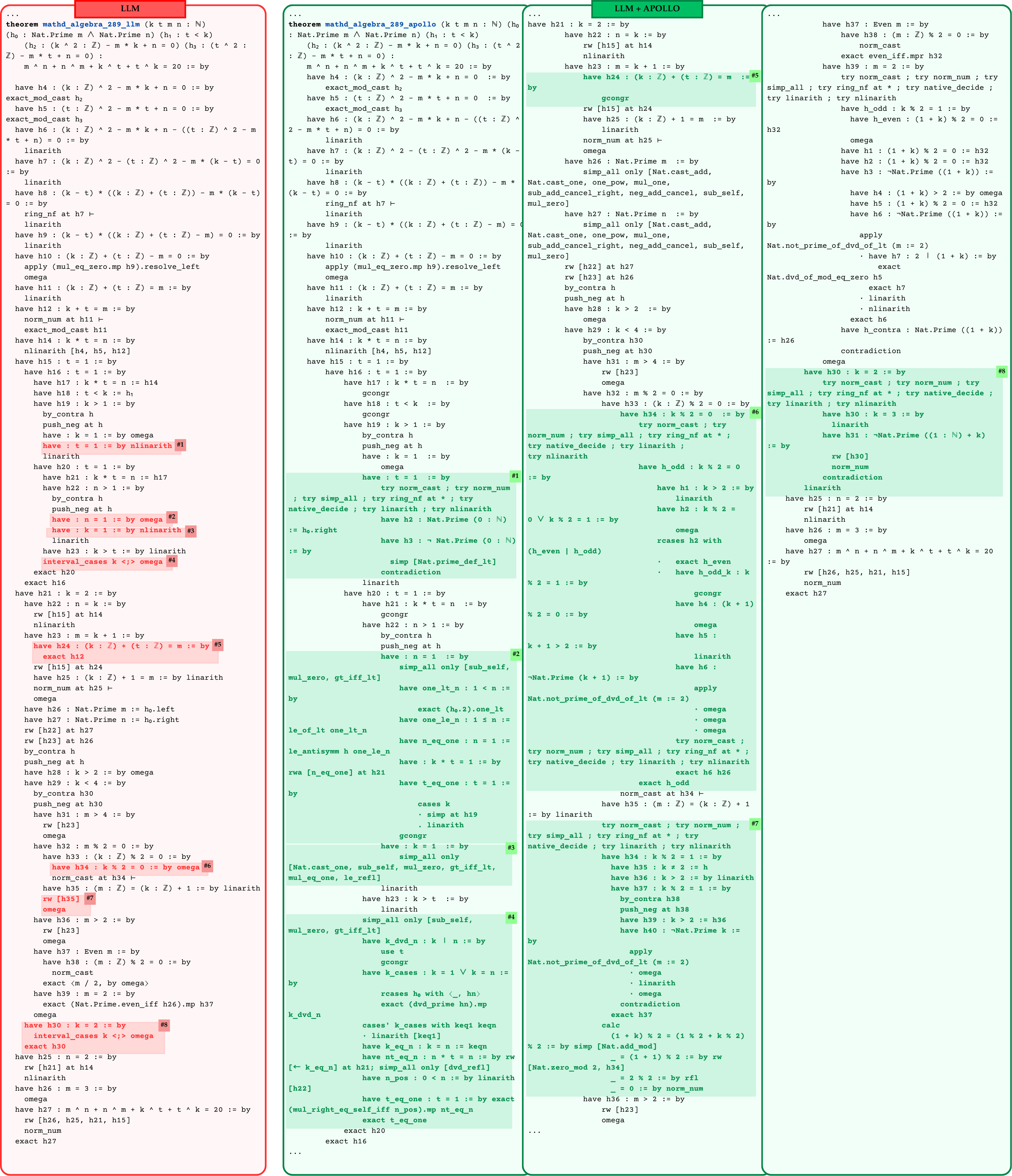
## Code Comparison Diagram: Lean 4 Theorem Proofs (LLM vs. LLM + APOLLO)
### Overview
The image displays a side-by-side comparison of three Lean 4 proof scripts for the same mathematical theorem (`mathd_algebra_289`). The leftmost column shows a proof generated by a base LLM, highlighted with red annotations. The middle and right columns show a proof generated by an LLM augmented with a system called "APOLLO," highlighted with green annotations. The comparison aims to demonstrate differences in proof strategy, tactic usage, and structure between the two methods.
### Components/Axes
The image is structured into three vertical columns, each with a header and a block of Lean 4 code.
1. **Column Headers (Top of each column):**
* **Left Column:** `LLM` (Red background, white text)
* **Middle Column:** `LLM + APOLLO` (Green background, white text)
* **Right Column:** `LLM + APOLLO` (Green background, white text)
2. **Code Blocks:** Each column contains a continuous block of Lean 4 code, starting with a `theorem` declaration and ending with `exact` or a similar concluding tactic. Lines within the code are annotated with colored highlights and numbered tags (e.g., `#1`, `#2`).
3. **Annotation System:**
* **Red Highlights (Left Column):** Indicate specific lines or steps in the base LLM proof. Each highlighted line has a small red tag with a number (e.g., `#1`, `#2`) on its right side.
* **Green Highlights (Middle & Right Columns):** Indicate corresponding or alternative steps in the APOLLO-augmented proof. Each highlighted line has a small green tag with a number (e.g., `#1`, `#2`) on its right side.
### Detailed Analysis
#### **Left Column: LLM Proof**
* **Theorem:** `theorem mathd_algebra_289_llm (k t m n : ℕ) (h₀ : Nat.Prime m ∧ Nat.Prime n) (h₁ : t < k) (h₂ : (k ^ 2 : ℤ) - m * k + n = 0) (h₃ : (t ^ 2 : ℤ) - m * t + n = 0) : m ^ n + n ^ m + k ^ t + t ^ k = 20 := by`
* **Proof Structure:** The proof proceeds through a series of `have` statements, introducing intermediate hypotheses (`h4` through `h27`). It uses tactics like `linarith`, `nlinarith`, `omega`, `ring_nf`, `norm_num`, `exact_mod_cast`, and `by_contra`.
* **Annotated (Red) Lines:**
* `#1`: `have : t = 1 := by nlinarith`
* `#2`: `have : n = 1 := by omega`
* `#3`: `have : k = 1 := by nlinarith`
* `#4`: `interval_cases k <;> omega`
* `#5`: `have h24 : (k : ℤ) + (t : ℤ) = m := by exact h12`
* `#6`: `have h34 : k % 2 = 0 := by omega`
* `#7`: `rw [h35]`
* `#8`: `have h30 : k = 2 := by interval_cases k <;> omega`
#### **Middle Column: LLM + APOLLO Proof (Part 1)**
* **Theorem:** `theorem mathd_algebra_289_apollo (k t m n : ℕ) (h₀ : Nat.Prime m ∧ Nat.Prime n) (h₁ : t < k) (h₂ : (k ^ 2 : ℤ) - m * k + n = 0) (h₃ : (t ^ 2 : ℤ) - m * t + n = 0) : m ^ n + n ^ m + k ^ t + t ^ k = 20 := by`
* **Proof Structure:** This proof also uses a sequence of `have` statements but employs a different set of tactics, often combining multiple tactics in a single step (e.g., `try norm_cast ; try norm_num ; try simp_all ; try ring_nf at * ; try native_decide ; try linarith ; try nlinarith`). It makes heavy use of `simp_all only [...]` with specific lemma lists.
* **Annotated (Green) Lines:**
* `#1`: `have : t = 1 := by try norm_cast ; try norm_num ; try simp_all ; try ring_nf at * ; try native_decide ; try linarith ; try nlinarith`
* `#2`: `have : n = 1 := by simp_all only [sub_self, mul_zero, gt_iff_lt]`
* `#3`: `have : k = 1 := by simp_all only [Nat.cast_one, sub_self, mul_zero, gt_iff_lt, mul_eq_one, le_refl]`
* `#4`: `simp_all only [sub_self, mul_zero, gt_iff_lt]`
#### **Right Column: LLM + APOLLO Proof (Part 2 - Continuation)**
* **Proof Structure:** This column continues the proof from the middle column. It introduces more hypotheses (`h21` through `h40`) and uses tactics like `gcongr`, `linarith`, `omega`, `rcases`, `apply`, `calc`, and `norm_num`.
* **Annotated (Green) Lines:**
* `#5`: `have h24 : (k : ℤ) + (t : ℤ) = m := by gcongr`
* `#6`: `have h34 : k % 2 = 0 := by try norm_cast ; try norm_num ; try simp_all ; try ring_nf at * ; try native_decide ; try linarith ; try nlinarith`
* `#7`: `try simp_all ; try norm_num ; try ring_nf at * ; try native_decide ; try linarith ; try nlinarith`
* `#8`: `have h30 : k = 2 := by try norm_cast ; try norm_num ; try simp_all ; try ring_nf at * ; try native_decide ; try linarith ; try nlinarith`
### Key Observations
1. **Proof Strategy Divergence:** The base LLM proof (red) relies heavily on arithmetic solvers (`linarith`, `nlinarith`, `omega`) and manual case analysis (`interval_cases`). The APOLLO-augmented proof (green) uses more structured simplification (`simp_all only [...]`) and broader, combined tactic blocks (`try ... ; try ...`).
2. **Tactic Specificity:** The APOLLO proof often specifies lists of lemmas for `simp_all` (e.g., `[sub_self, mul_zero, gt_iff_lt]`), suggesting a more targeted simplification approach. The base LLM proof uses more generic arithmetic tactics.
3. **Annotation Correspondence:** The numbered annotations (`#1` through `#8`) appear to mark analogous steps or decision points in the two proofs, allowing for direct comparison of how each method handles the same logical subgoal.
4. **Code Density:** The APOLLO proof columns appear slightly denser, with more complex single-line tactic calls, while the base LLM proof has more discrete, single-tactic lines.
### Interpretation
This diagram is a technical comparison designed to evaluate the performance of an AI system ("APOLLO") that assists or augments a base Large Language Model (LLM) in generating formal mathematical proofs in Lean 4.
* **What the data suggests:** The comparison implies that the APOLLO system guides the LLM towards a different, potentially more robust or systematic proof strategy. The use of targeted simplification (`simp_all` with specific lemmas) and combined tactic blocks may lead to proofs that are less reliant on brute-force arithmetic solving and more on algebraic simplification and logical structure.
* **How elements relate:** The red and green highlights create a direct visual mapping between corresponding proof steps. This allows a reviewer to assess not just the final output, but the *process*—how each system arrives at intermediate conclusions like `t = 1`, `n = 1`, or `k = 2`.
* **Notable patterns/anomalies:** The most striking pattern is the shift from sequential, single-tactic reasoning in the LLM column to bundled, multi-tactic attempts in the APOLLO columns. This could indicate that APOLLO promotes a "try everything relevant" approach at key junctures, which might be more successful in navigating complex proof states. The absence of `interval_cases` in the annotated APOLLO steps (compared to its use in LLM steps `#4` and `#8`) is a notable strategic difference, suggesting APOLLO finds alternative paths to the same conclusions.
**Language Note:** The code is written in the **Lean 4** programming language and proof assistant. All comments, tactic names, and syntax are part of this formal language. The theorem statement and proof steps are in mathematical logic expressed through Lean's syntax.
DECODING INTELLIGENCE...