## Laplace Transform Properties: Time Domain Operations
### Overview
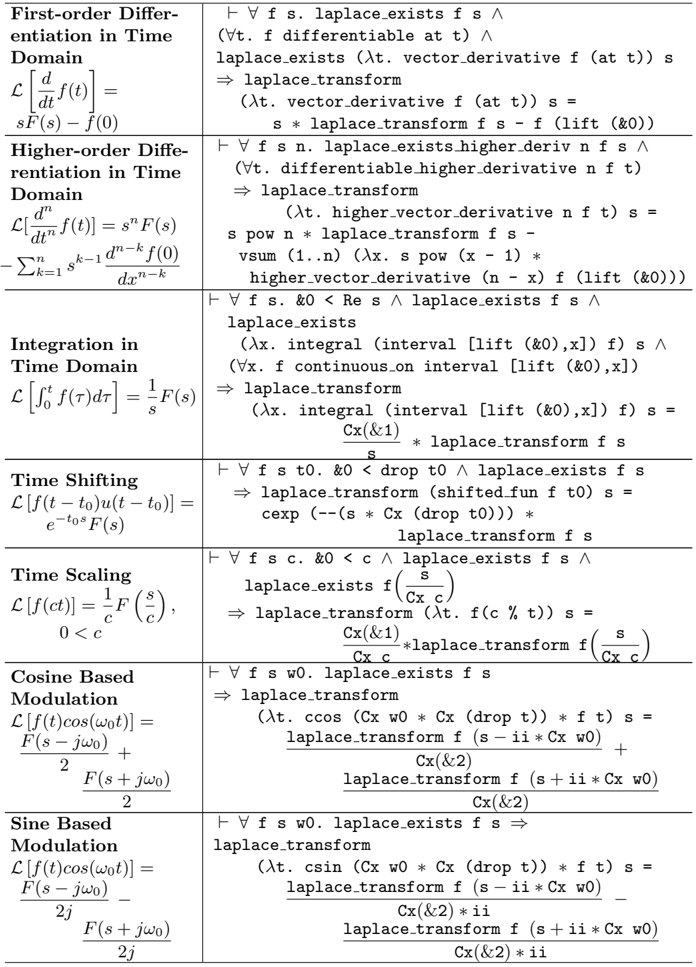
The image presents a table summarizing several properties of the Laplace transform related to operations performed in the time domain. It includes formulas for differentiation, integration, time shifting, time scaling, and modulation (cosine and sine). Each property is presented with its corresponding Laplace transform and any necessary conditions.
### Components/Axes
The table is structured with the following columns:
1. **Operation Description**: Describes the operation performed on the function in the time domain (e.g., "First-order Differentiation in Time Domain").
2. **Laplace Transform**: Provides the formula for the Laplace transform of the modified function, denoted as L[f(t)] = F(s).
3. **Conditions/Mathematical Expressions**: Specifies the conditions under which the property holds, often involving quantifiers and logical statements.
### Detailed Analysis or ### Content Details
Here's a breakdown of each row:
1. **First-order Differentiation in Time Domain**
* **Description**: Deals with the Laplace transform of the derivative of a function.
* **Laplace Transform**: L[d/dt f(t)] = sF(s) - f(0)
* **Conditions**: ∀ f s. laplace\_exists f s ∧ (∀t. f differentiable at t) ∧ laplace\_exists (λt. vector\_derivative f (at t)) s ⇒ laplace\_transform (λt. vector\_derivative f (at t)) s = s \* laplace\_transform f s - f (lift (&0))
2. **Higher-order Differentiation in Time Domain**
* **Description**: Deals with the Laplace transform of the nth derivative of a function.
* **Laplace Transform**: L[d^n/dt^n f(t)] = s^n F(s) - Σ{k=1 to n} s^(k-1) d^(n-k)/dx^(n-k) f(0)
* **Conditions**: ∀ f s n. laplace\_exists\_higher\_deriv n f s ∧ (∀t. differentiable higher\_derivative n f t) ⇒ laplace\_transform (λt. higher\_vector\_derivative n f t) s = s pow n \* laplace\_transform f s - vsum (1..n) (λx. s pow (x - 1) \* higher\_vector\_derivative (n - x) f (lift (&0)))
3. **Integration in Time Domain**
* **Description**: Deals with the Laplace transform of the integral of a function.
* **Laplace Transform**: L[∫{0 to t} f(τ) dτ] = (1/s) F(s)
* **Conditions**: ∀ f s. &0 < Re s ∧ laplace\_exists f s ∧ laplace\_exists (λx. integral (interval [lift (&0),x]) f) s ∧ (∀x. f continuous\_on interval [lift (&0),x]) ⇒ laplace\_transform (λx. integral (interval [lift (&0),x]) f) s = Cx(&1)/s \* laplace\_transform f s
4. **Time Shifting**
* **Description**: Deals with the Laplace transform of a time-shifted function.
* **Laplace Transform**: L[f(t - t0)u(t - t0)] = e^(-t0s) F(s)
* **Conditions**: ∀ f s t0. &0 < drop t0 ∧ laplace\_exists f s ⇒ laplace\_transform (shifted\_fun f t0) s = cexp (-- (s \* Cx (drop t0))) \* laplace\_transform f s
5. **Time Scaling**
* **Description**: Deals with the Laplace transform of a time-scaled function.
* **Laplace Transform**: L[f(ct)] = (1/c) F(s/c), 0 < c
* **Conditions**: ∀ f s c. &0 < c ∧ laplace\_exists f s ∧ laplace\_exists f(s/Cx c) ⇒ laplace\_transform (λt. f(c % t)) s = Cx(&1)/(Cx c) \* laplace\_transform f(s/Cx c)
6. **Cosine Based Modulation**
* **Description**: Deals with the Laplace transform of a function multiplied by a cosine.
* **Laplace Transform**: L[f(t)cos(ω0t)] = F(s - jω0)/2 + F(s + jω0)/2
* **Conditions**: ∀ f s w0. laplace\_exists f s ⇒ laplace\_transform (λt. ccos (Cx w0 \* Cx (drop t)) \* f t) s = laplace\_transform f (s - ii \* Cx w0) / Cx(&2) + laplace\_transform f (s + ii \* Cx w0) / Cx(&2)
7. **Sine Based Modulation**
* **Description**: Deals with the Laplace transform of a function multiplied by a sine.
* **Laplace Transform**: L[f(t)cos(ω0t)] = F(s - jω0)/(2j) - F(s + jω0)/(2j)
* **Conditions**: ∀ f s w0. laplace\_exists f s ⇒ laplace\_transform (λt. csin (Cx w0 \* Cx (drop t)) \* f t) s = laplace\_transform f (s - ii \* Cx w0) / (Cx(&2) \* ii) - laplace\_transform f (s + ii \* Cx w0) / (Cx(&2) \* ii)
### Key Observations
* The table provides a concise summary of how time-domain operations affect the Laplace transform of a function.
* Each property is accompanied by conditions that must be met for the property to hold.
* The modulation properties (cosine and sine) involve complex numbers (j or ii, representing the imaginary unit).
### Interpretation
The table serves as a reference for engineers and scientists who use Laplace transforms to analyze and solve differential equations and other problems in linear systems. It demonstrates how operations in the time domain (differentiation, integration, shifting, scaling, and modulation) translate into corresponding operations in the s-domain (Laplace domain), which can simplify the analysis and solution of complex systems. The conditions specified for each property ensure the validity of the transform.