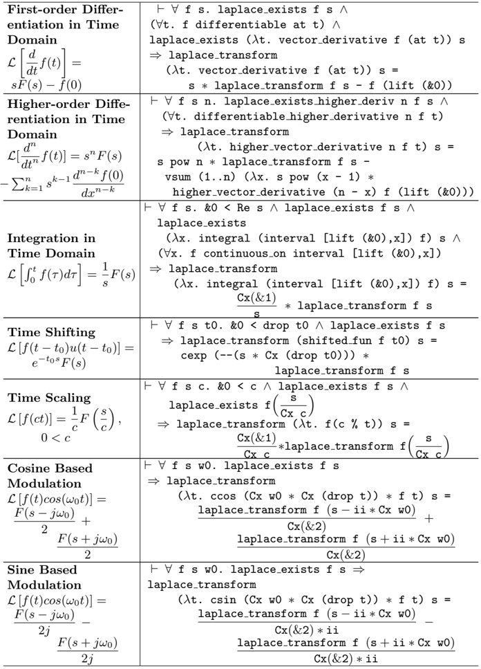
## Mathematical Diagram: Table of Laplace Transform Properties and Formal Specifications ### Overview The image displays a two-column table presenting seven key properties of the Laplace transform. The left column provides the standard mathematical notation for each property, while the right column contains corresponding formal logic statements, likely written in a proof assistant language (such as Isabelle/HOL or a similar formal verification framework). The table serves as a reference for both the conventional mathematical formulation and its machine-verifiable counterpart. ### Components/Axes The content is organized into a table with two primary columns and seven rows, each dedicated to a specific property. * **Left Column:** Contains the property name (e.g., "First-order Differentiation in Time Domain") and the standard Laplace transform formula using conventional mathematical notation. * **Right Column:** Contains a formal logic statement beginning with a turnstile symbol (`⊢`), followed by a series of quantified conditions (`∀`, `∧`) and an implication (`⇒`) leading to the formal definition of the `laplace_transform` for that property. * **Rows (Properties):** 1. First-order Differentiation in Time Domain 2. Higher-order Differentiation in Time Domain 3. Integration in Time Domain 4. Time Shifting 5. Time Scaling 6. Cosine Based Modulation 7. Sine Based Modulation ### Detailed Analysis Below is the precise transcription of each row's content. **Row 1: First-order Differentiation in Time Domain** * **Left (Standard Formula):** `L[ d/dt f(t) ] = sF(s) - f̃(0)` * **Right (Formal Statement):** `⊢ ∀ f s. laplace_exists f s ∧ (∀t. f differentiable at t) ∧ laplace_exists (λt. vector_derivative f (at t)) s ⇒ laplace_transform (λt. vector_derivative f (at t)) s = s * laplace_transform f s - f (lift (&0))` **Row 2: Higher-order Differentiation in Time Domain** * **Left (Standard Formula):** `L[ dⁿ/dtⁿ f(t) ] = sⁿF(s) - Σₖ₌₁ⁿ sᵏ⁻¹ * (dⁿ⁻ᵏf(0)/dxⁿ⁻ᵏ)` * **Right (Formal Statement):** `⊢ ∀ f s n. laplace_exists.higher_deriv n f s ∧ (∀t. differentiable.higher_derivative n f t) ⇒ laplace_transform (λt. higher_vector_derivative n f t) s = s pow n * laplace_transform f s - vsum (1..n) (λx. s pow (x - 1) * higher_vector_derivative (n - x) f (lift (&0)))` **Row 3: Integration in Time Domain** * **Left (Standard Formula):** `L[ ∫₀ᵗ f(τ)dτ ] = (1/s) F(s)` * **Right (Formal Statement):** `⊢ ∀ f s. &0 < Re s ∧ laplace_exists f s ∧ laplace_exists (λx. integral (interval [lift (&0),x]) f) s ∧ (∀x. f continuous_on interval [lift (&0),x]) ⇒ laplace_transform (λx. integral (interval [lift (&0),x]) f) s = (Cx(&1) / s) * laplace_transform f s` **Row 4: Time Shifting** * **Left (Standard Formula):** `L[ f(t - t₀)u(t - t₀) ] = e^(-t₀s) F(s)` * **Right (Formal Statement):** `⊢ ∀ f s t0. &0 < drop t0 ∧ laplace_exists f s ⇒ laplace_transform (shifted_fun f t0) s = cexp (-(s * Cx (drop t0))) * laplace_transform f s` **Row 5: Time Scaling** * **Left (Standard Formula):** `L[ f(ct) ] = (1/c) F(s/c), 0 < c` * **Right (Formal Statement):** `⊢ ∀ f s c. &0 < c ∧ laplace_exists f s ∧ laplace_exists f (s / Cx c) ⇒ laplace_transform (λt. f(c * t)) s = (Cx(&1) / Cx c) * laplace_transform f (s / Cx c)` **Row 6: Cosine Based Modulation** * **Left (Standard Formula):** `L[ f(t)cos(ω₀t) ] = [F(s - jω₀) + F(s + jω₀)] / 2` * **Right (Formal Statement):** `⊢ ∀ f s w0. laplace_exists f s ⇒ laplace_transform (λt. ccos (Cx w0 * Cx (drop t)) * f t) s = (laplace_transform f (s - ii * Cx w0) / Cx(&2)) + (laplace_transform f (s + ii * Cx w0) / Cx(&2))` **Row 7: Sine Based Modulation** * **Left (Standard Formula):** `L[ f(t)sin(ω₀t) ] = [F(s - jω₀) - F(s + jω₀)] / 2j` * **Right (Formal Statement):** `⊢ ∀ f s w0. laplace_exists f s ⇒ laplace_transform (λt. csin (Cx w0 * Cx (drop t)) * f t) s = (laplace_transform f (s - ii * Cx w0) / (Cx(&2) * ii)) - (laplace_transform f (s + ii * Cx w0) / (Cx(&2) * ii))` ### Key Observations 1. **Dual Representation:** Each property is presented in two distinct formalisms: the familiar engineering/physics notation and a rigorous, machine-oriented logical specification. 2. **Formal Language Syntax:** The right column uses a consistent syntax featuring quantifiers (`∀`), logical conjunction (`∧`), implication (`⇒`), lambda expressions (`λ`), and specific function names (`laplace_transform`, `vector_derivative`, `integral`, `cexp`, `ccos`, `csin`). 3. **Preconditions:** The formal statements explicitly include necessary preconditions for the transform's existence (`laplace_exists`), differentiability, and continuity, which are often implied in standard textbook presentations. 4. **Complexity Gradient:** The formulas increase in complexity from simple differentiation to integral properties and modulation theorems. The formal statements for integration and higher-order differentiation are notably more verbose. ### Interpretation This table is a bridge between applied mathematics and formal verification. Its primary purpose is to provide a definitive, unambiguous reference for the Laplace transform properties that can be used both by humans for study and by computer systems for proof checking or symbolic computation. * **Relationship Between Columns:** The left column is the "what" – the result engineers and physicists use. The right column is the "how" – the precise logical foundation that guarantees the result is correct under specified conditions. The formal statements essentially encode the theorems in a language a proof assistant can process. * **Significance:** Such a resource is critical in fields requiring high assurance, like formal methods for control system design or the verification of signal processing algorithms. It ensures that the mathematical transformations applied in software are theoretically sound. * **Notable Pattern:** The formalization reveals the underlying structure more explicitly. For example, the "Time Shifting" property uses a `shifted_fun` function, and modulation uses complex trigonometric functions (`ccos`, `csin`), making the operations on the complex plane explicit. The use of `Cx` likely denotes embedding a real number into the complex plane. * **Anomaly/Observation:** The standard formula for "Sine Based Modulation" in the left column contains a likely typo: it writes `cos(ω₀t)` instead of `sin(ω₀t)` in the `L[...]` operator, though the right-hand side of the equation correctly uses the sine form. The formal statement on the right correctly uses `csin`.