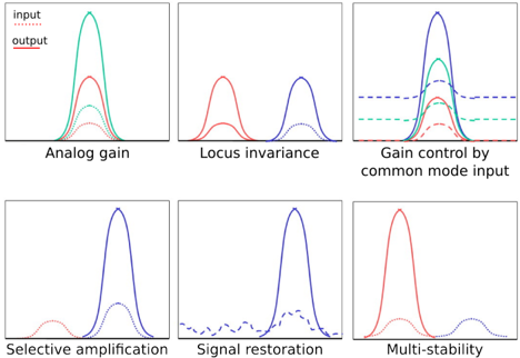
## Chart Type: Comparative Response Curves ### Overview The image presents six separate plots, each illustrating the relationship between an "input" signal and the resulting "output" signal under different conditions or system configurations. Each plot shows response curves, with the x-axis representing the input signal strength or frequency (unspecified, but assumed to be consistent across plots), and the y-axis representing the output signal strength. The plots are arranged in a 2x3 grid. ### Components/Axes * **X-axis:** Implicitly represents the input signal characteristic (e.g., strength, frequency). No explicit scale is provided. * **Y-axis:** Represents the output signal strength. No explicit scale is provided. * **Legend (Top-Left of the first plot):** * `input`: Represented by dotted lines, typically in red or blue. * `output`: Represented by solid lines, typically in red, blue, or green. * **Plot Titles (Below each plot):** * Analog gain * Locus invariance * Gain control by common mode input * Selective amplification * Signal restoration * Multi-stability ### Detailed Analysis **1. Analog Gain (Top-Left)** * **Input:** Several dotted red lines, each representing a different input level. The peaks of these curves increase from left to right. * **Output:** A solid green line, showing a single peak. The peak is significantly higher than any of the input peaks. * **Trend:** The analog gain plot shows that the output signal is amplified relative to the input signal. The amplification factor appears to be non-linear, as the output peak is much larger than the largest input peak. **2. Locus Invariance (Top-Middle)** * **Input:** Not explicitly shown, but implied. * **Output:** Two solid red lines, each showing a single peak. The peaks are separated along the x-axis. * **Trend:** The locus invariance plot suggests that the system responds to two distinct input locations or frequencies, producing two separate output peaks. **3. Gain Control by Common Mode Input (Top-Right)** * **Input:** A dotted red line with a single peak and a dashed blue line that is relatively flat. * **Output:** A solid blue line with a single peak, and a solid green line with a single peak. The green peak is slightly lower than the blue peak. A dashed green line is also present, with a single peak. * **Trend:** This plot shows how a common mode input (represented by the dashed blue line) can influence the gain of the system. The output signal varies depending on the presence and characteristics of the common mode input. **4. Selective Amplification (Bottom-Left)** * **Input:** A dotted red line with two small peaks. * **Output:** A solid blue line with a single, large peak. * **Trend:** The selective amplification plot indicates that the system amplifies only one of the input signals, suppressing the other. **5. Signal Restoration (Bottom-Middle)** * **Input:** A dashed blue line with multiple small oscillations. * **Output:** A solid blue line with a single, large peak. * **Trend:** The signal restoration plot demonstrates the system's ability to reconstruct a clean signal from a noisy or distorted input. **6. Multi-Stability (Bottom-Right)** * **Input:** A dotted red line with two small peaks. * **Output:** A solid red line with a single, large peak. * **Trend:** The multi-stability plot suggests that the system can maintain a stable output state even with multiple potential input signals. ### Key Observations * Each plot demonstrates a different type of signal processing or system behavior. * The "input" and "output" signals are represented by different line styles (dotted vs. solid) and colors. * The plots lack explicit scales on the x and y axes, making it difficult to quantify the relationships between input and output signals. ### Interpretation The image illustrates various signal processing concepts, such as amplification, filtering, and signal restoration. Each plot demonstrates a specific functionality or characteristic of a system in response to different input signals. The absence of explicit scales limits the quantitative analysis, but the qualitative relationships between input and output signals are clearly depicted. The plots suggest that the system can perform a variety of signal processing tasks, including amplifying specific signals, suppressing noise, and maintaining stable output states. The "Gain control by common mode input" plot highlights the importance of considering common mode signals in system design.

\n ## Diagram: Neural Network Response Characteristics ### Overview The image presents a 2x3 grid of diagrams illustrating different response characteristics of a neural network or similar system. Each diagram depicts a distribution or curve, likely representing signal strength or activation level, with different curves representing "input" and "output" signals. The diagrams are labeled with descriptive titles indicating the specific characteristic being demonstrated. There are no explicit axes labels or numerical values provided. ### Components/Axes Each sub-diagram contains curves representing input and output signals. The legend, consistently positioned in the top-left corner of each diagram, indicates: * **input** (represented by a dotted blue line) * **output** (represented by a solid red or teal line). The diagrams are labeled as follows (from top-left to bottom-right): 1. Analog gain 2. Locus invariance 3. Gain control by common mode input 4. Selective amplification 5. Signal restoration 6. Multi-stability ### Detailed Analysis or Content Details **1. Analog Gain:** The "input" (dotted blue) is a relatively broad distribution. The "output" (solid teal) is a narrower, taller distribution centered around the same point, indicating amplification. A smaller red curve is also present, likely representing another output. **2. Locus Invariance:** The "input" (dotted blue) is a relatively narrow distribution. The "output" (solid red) is a similar distribution, but shifted slightly to the right. **3. Gain Control by Common Mode Input:** The "input" (dotted blue) is a broad distribution. There are multiple "output" curves (solid teal, dashed blue, and dashed red). The solid teal curve is the tallest and narrowest, indicating high gain. The dashed curves are lower and broader, suggesting gain control based on a common mode input. **4. Selective Amplification:** The "input" (dotted blue) is a broad distribution. The "output" (solid red) is a narrow, tall distribution centered on a specific point within the input distribution, indicating selective amplification. **5. Signal Restoration:** The "input" (dotted blue) is a noisy, low-amplitude distribution. The "output" (solid red) is a cleaner, higher-amplitude distribution, suggesting signal restoration. A dashed blue curve is also present, representing an intermediate signal. **6. Multi-stability:** There are two distinct "output" curves (solid red and solid blue), each representing a stable state. The "input" (dotted blue) is a broad distribution, suggesting the system can settle into either of the two stable states depending on the input. ### Key Observations * The diagrams visually demonstrate different functional properties of a system, likely a neural network or similar signal processing unit. * The "output" curves are consistently modified versions of the "input" curves, illustrating the system's transformation of the input signal. * There is a consistent use of color coding (blue for input, red/teal for output) across all diagrams. * No quantitative data is provided; the diagrams are purely illustrative. ### Interpretation The image serves as a conceptual overview of various response characteristics achievable in a neural network or similar system. Each diagram highlights a specific function: amplification, invariance, gain control, selective processing, signal recovery, and multi-stability. The absence of numerical data suggests the diagrams are intended to convey qualitative understanding rather than precise quantitative relationships. The diagrams are likely used in a teaching or explanatory context to illustrate the capabilities of such systems. The consistent use of "input" and "output" curves allows for a direct comparison of how the system modifies the input signal to produce the output. The "Gain control by common mode input" diagram suggests a mechanism for regulating signal strength based on external factors. The "Multi-stability" diagram indicates the system can exhibit multiple stable states, potentially enabling memory or complex decision-making.

## Diagram: Signal Processing/Neural Response Patterns ### Overview The image displays a 2x3 grid of six individual plots, each illustrating a different principle of signal transformation or neural response. Each plot contains multiple curves representing input signals (dashed lines) and output signals (solid lines) of varying amplitudes and positions. A legend in the top-left plot defines the line styles. ### Components/Axes * **Legend:** Located in the top-left corner of the first subplot ("Analog gain"). * `input`: Represented by dashed lines (`---`). * `output`: Represented by solid lines (`—`). * **Plot Titles:** Each of the six subplots has a centered title below its graph: 1. Analog gain 2. Locus invariance 3. Gain control by common mode input 4. Selective amplification 5. Signal restoration 6. Multi-stability * **Axes:** The plots do not have explicit numerical axis labels or titles. The horizontal axis likely represents a variable such as time, stimulus intensity, or spatial position. The vertical axis represents signal amplitude or response magnitude. * **Color Palette:** Four distinct colors are used for the curves: teal/green, red, blue, and purple. ### Detailed Analysis **1. Analog gain (Top-Left)** * **Components:** Three pairs of curves (teal, red, blue). Each pair consists of a dashed input curve and a solid output curve of the same color. * **Trend/Relationship:** The output curves are scaled versions of their corresponding input curves. The peak amplitude of the output is directly proportional to the peak amplitude of the input. The teal input has the highest peak, followed by red, then blue, and the outputs maintain this exact order and relative scaling. * **Spatial Grounding:** The curves are centered on the plot. The teal curves have the highest amplitude, red is in the middle, and blue is the lowest. **2. Locus invariance (Top-Center)** * **Components:** Two pairs of curves (red, blue). Each pair has a dashed input and a solid output. * **Trend/Relationship:** The input curves (dashed) are positioned at different locations along the horizontal axis (red left, blue right). The output curves (solid) are both centered at the same, central location, regardless of where their corresponding input was. The shape and amplitude of the outputs appear similar. * **Spatial Grounding:** The red input is left-of-center, the blue input is right-of-center. Both solid output peaks are aligned in the center of the plot. **3. Gain control by common mode input (Top-Right)** * **Components:** Multiple curves. Three solid output curves (purple, teal, red) and three dashed horizontal lines (purple, teal, red) representing baseline or "common mode" input levels. * **Trend/Relationship:** The amplitude of the output peaks is inversely related to the level of the corresponding dashed baseline input. The purple baseline is highest, and its corresponding purple output peak is the smallest. The red baseline is lowest, and its red output peak is the largest. The teal baseline and output peak are intermediate. * **Spatial Grounding:** The dashed baseline lines are horizontal and stacked vertically (purple top, teal middle, red bottom). The solid output peaks are centered and stacked in reverse order (red tallest, teal middle, purple shortest). **4. Selective amplification (Bottom-Left)** * **Components:** Two pairs of curves (blue, red). * **Trend/Relationship:** The blue input curve (dashed) has a moderate amplitude. Its corresponding blue output curve (solid) is dramatically amplified, showing a very high, sharp peak. The red input curve (dashed) has a smaller amplitude, and its red output curve (solid) is only slightly amplified or remains similar. The system selectively amplifies the stronger input signal. * **Spatial Grounding:** The blue curves are centered and dominant. The red curves are smaller and positioned to the left. **5. Signal restoration (Bottom-Center)** * **Components:** One dashed blue input curve and one solid blue output curve. * **Trend/Relationship:** The input signal (dashed) is low-amplitude and appears noisy or irregular. The output signal (solid) is a clean, high-amplitude, smooth bell-shaped curve. The system transforms a weak, noisy input into a strong, clean, stereotypical output. * **Spatial Grounding:** Both curves are centered. The output peak is significantly taller and smoother than the input. **6. Multi-stability (Bottom-Right)** * **Components:** Two pairs of curves (red, blue). * **Trend/Relationship:** The system produces two distinct, stable output states (solid lines) from inputs (dashed lines) of similar, low amplitude. The red input yields a high-amplitude red output peak. The blue input yields a low-amplitude blue output peak. The outputs are bistable, settling into one of two very different response magnitudes. * **Spatial Grounding:** The red output peak is tall and centered. The blue output peak is short and positioned to the right. ### Key Observations * **Consistent Coding:** The color of a dashed input curve always matches the color of its corresponding solid output curve. * **Nonlinear Transformations:** None of the plots show a simple 1:1 linear relationship. All demonstrate nonlinear transformations: scaling, translation, normalization, selective amplification, denoising, and bistability. * **Absence of Quantitative Data:** The plots are conceptual. No numerical values are provided on the axes, making precise data extraction impossible. The analysis is based on relative comparisons of shape, position, and amplitude. ### Interpretation This diagram serves as a conceptual toolkit illustrating fundamental computational principles likely relevant to neuroscience, sensor systems, or nonlinear signal processing. Each panel demonstrates a specific functional capability: 1. **Analog gain** shows faithful, proportional signal relay. 2. **Locus invariance** demonstrates position-independent recognition or normalization. 3. **Gain control by common mode input** depicts adaptive normalization, where the system's sensitivity is adjusted by a background signal, preventing saturation. 4. **Selective amplification** illustrates a thresholding or attentional mechanism, boosting relevant signals while suppressing weaker ones. 5. **Signal restoration** shows denoising and pattern completion, recovering a canonical signal from corrupted input. 6. **Multi-stability** reveals a system with discrete attractor states, capable of making binary decisions or maintaining memory from similar inputs. Together, these principles describe a system that is not a passive relay but an active processor. It normalizes, filters, amplifies, and categorizes incoming information, transforming raw inputs into structured, meaningful, and robust representations. This is characteristic of biological neural networks and advanced engineered systems designed for perception and decision-making in noisy environments. The lack of quantitative data emphasizes that these are general, qualitative properties of a class of nonlinear systems.

## Line Graphs: Signal Processing Mechanisms ### Overview The image consists of six line graphs arranged in two rows of three panels. Each panel illustrates a distinct signal processing mechanism, with colored curves representing different data series. The graphs emphasize relationships between input/output signals, gain control, and stability phenomena. ### Components/Axes - **X-Axes**: - Panel 1: "Analog gain" - Panel 2: "Locus invariance" - Panel 3: "Gain control by common mode input" - Panel 4: "Selective amplification" - Panel 5: "Signal restoration" - Panel 6: "Multi-stability" - **Y-Axes**: All panels share the label "Output" (except Panel 2, which may have an implicit "Output" label based on context). - **Legends**: No explicit legend is visible in the image. Colors and line styles are inferred from curve descriptions. ### Detailed Analysis 1. **Analog gain** - **Curves**: - Red (solid): "Output" (peaks at ~1.2 on y-axis) - Blue (dashed): "Input" (peaks at ~0.8 on y-axis) - Green (dotted): Intermediate curve (peaks at ~1.0 on y-axis) - **Trend**: Output (red) exceeds input (blue), with green curve showing a moderate response. 2. **Locus invariance** - **Curves**: - Red (solid): Peaks at ~1.1 on y-axis - Blue (dashed): Peaks at ~0.9 on y-axis - **Trend**: Red curve dominates, suggesting higher output stability under varying locus conditions. 3. **Gain control by common mode input** - **Curves**: - Blue (solid): Peaks at ~1.3 on y-axis - Green (dashed): Peaks at ~1.1 on y-axis - Red (dotted): Peaks at ~0.9 on y-axis - **Trend**: Blue curve (highest gain) is followed by green and red, indicating tiered gain control. 4. **Selective amplification** - **Curves**: - Red (solid): Peaks at ~1.4 on y-axis - Blue (dashed): Peaks at ~0.7 on y-axis - **Trend**: Red curve (amplified signal) is significantly higher than blue (unamplified). 5. **Signal restoration** - **Curves**: - Blue (solid): Peaks at ~1.5 on y-axis - Red (dashed): Peaks at ~0.5 on y-axis - **Trend**: Blue curve (restored signal) is sharply higher than red (degraded signal). 6. **Multi-stability** - **Curves**: - Red (solid): Peaks at ~1.6 on y-axis - Blue (dashed): Peaks at ~0.6 on y-axis - **Trend**: Red curve (stable state) dominates, with blue curve (unstable state) showing lower output. ### Key Observations - **Output Dominance**: In all panels, the solid-colored curves (e.g., red, blue) consistently exceed dashed/dotted curves, indicating amplified or stabilized outputs. - **Color Coding**: Red often represents "output" or "stable" states, while blue/blue-dashed curves denote "input" or "unstable" states. Green curves (e.g., Panel 1, 3) act as intermediaries. - **Peak Values**: Output peaks range from ~0.5 to ~1.6 on the y-axis, with no explicit numerical scale provided. ### Interpretation The graphs collectively illustrate how signal processing mechanisms modulate input signals to achieve desired outputs. For example: - **Analog gain** and **gain control by common mode input** highlight how amplification levels vary with input conditions. - **Locus invariance** and **multi-stability** suggest system stability under different operational parameters. - **Selective amplification** and **signal restoration** emphasize targeted enhancement or recovery of signals. The absence of a legend introduces ambiguity in color assignments, but the consistent use of red for "output" and blue for "input" across panels implies a standardized convention. The graphs likely model scenarios in analog electronics, control systems, or signal processing, where gain, stability, and signal fidelity are critical.