\n
## Histogram: Distribution of Token Counts in a Dataset
### Overview
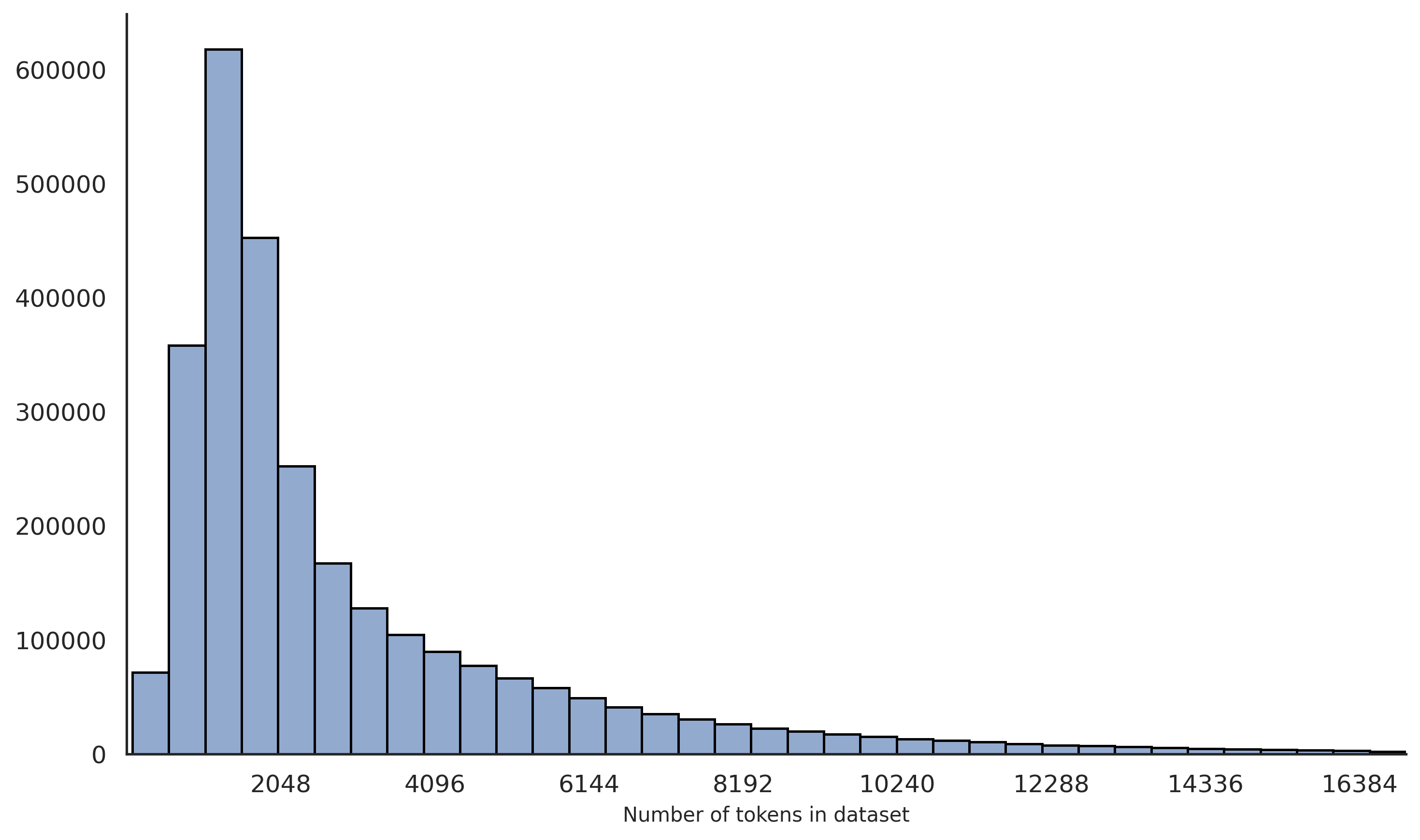
The image presents a histogram visualizing the distribution of the number of tokens in a dataset. The x-axis represents the number of tokens, and the y-axis represents the frequency (count) of datasets with that number of tokens. The histogram shows a heavily right-skewed distribution, indicating that most datasets have a relatively small number of tokens, while a few datasets have a very large number of tokens.
### Components/Axes
* **X-axis Label:** "Number of tokens in dataset"
* **Y-axis Label:** (Implied) Frequency or Count
* **X-axis Scale:** The x-axis is scaled linearly, with markers at 2048, 4096, 6144, 8192, 10240, 12288, 14336, and 16384.
* **Y-axis Scale:** The y-axis is scaled linearly, starting at 0 and going up to approximately 600,000.
* **Histogram Bars:** The histogram consists of a series of bars, each representing a range of token counts.
### Detailed Analysis
The histogram displays the following approximate data points (reading from left to right):
* **2048 tokens:** Approximately 600,000 datasets. This is the highest frequency.
* **2560 tokens:** Approximately 550,000 datasets.
* **3072 tokens:** Approximately 480,000 datasets.
* **3584 tokens:** Approximately 420,000 datasets.
* **4096 tokens:** Approximately 350,000 datasets.
* **4608 tokens:** Approximately 290,000 datasets.
* **5120 tokens:** Approximately 240,000 datasets.
* **5632 tokens:** Approximately 190,000 datasets.
* **6144 tokens:** Approximately 150,000 datasets.
* **6656 tokens:** Approximately 120,000 datasets.
* **7168 tokens:** Approximately 90,000 datasets.
* **7680 tokens:** Approximately 70,000 datasets.
* **8192 tokens:** Approximately 50,000 datasets.
* **8704 tokens:** Approximately 40,000 datasets.
* **9216 tokens:** Approximately 30,000 datasets.
* **9728 tokens:** Approximately 20,000 datasets.
* **10240 tokens:** Approximately 15,000 datasets.
* **10752 tokens:** Approximately 10,000 datasets.
* **11264 tokens:** Approximately 8,000 datasets.
* **11776 tokens:** Approximately 6,000 datasets.
* **12288 tokens:** Approximately 4,000 datasets.
* **12800 tokens:** Approximately 3,000 datasets.
* **13312 tokens:** Approximately 2,000 datasets.
* **13824 tokens:** Approximately 1,500 datasets.
* **14336 tokens:** Approximately 1,000 datasets.
* **14848 tokens:** Approximately 700 datasets.
* **15360 tokens:** Approximately 500 datasets.
* **15872 tokens:** Approximately 300 datasets.
* **16384 tokens:** Approximately 200 datasets.
The histogram bars generally decrease in height as the number of tokens increases. The decline is steepest in the lower range of token counts (2048-8192) and becomes more gradual as the token count increases.
### Key Observations
* The distribution is highly skewed to the right.
* The majority of datasets have fewer than 4096 tokens.
* There is a long tail of datasets with a large number of tokens, though their frequency is much lower.
* The frequency decreases almost exponentially with increasing token count.
### Interpretation
This histogram suggests that the dataset consists of many small documents or data entries, with a few exceptionally large ones. This could be due to a variety of factors, such as:
* **Natural Language Processing:** The dataset might be a collection of text documents, where most documents are short (e.g., tweets, short articles) and a few are very long (e.g., books, long reports).
* **Data Logging:** The dataset might be a log of events, where most events are simple and a few are complex and generate a lot of data.
* **Data Aggregation:** The dataset might be aggregated from multiple sources, where some sources produce more data than others.
The right skew indicates that the average token count is likely to be higher than the median token count. The long tail suggests that the presence of these larger datasets could significantly impact any analysis that is sensitive to outliers (e.g., calculating the average token count). Further investigation might be needed to understand the nature of these large datasets and whether they should be treated differently in the analysis.