## [Line Graphs]: Prior Function Approximation Comparison
### Overview
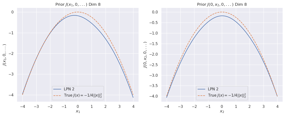
The image displays two side-by-side line graphs comparing an approximated function ("LPN 2") against a true mathematical function ("True J(x)") in an 8-dimensional space. The graphs plot the value of a function `J` against a single variable (`x₁` or `x₂`) while holding other dimensions at zero.
### Components/Axes
* **Chart Type:** Two 2D line plots.
* **Titles:**
* Left Plot: `Prior J(x₁, 0, ...) Dim 8`
* Right Plot: `Prior J(0, x₂, 0, ...) Dim 8`
* **Axes:**
* **X-Axis (Left Plot):** Labeled `x₁`. Scale ranges from -4 to 4 with major ticks at -4, -3, -2, -1, 0, 1, 2, 3, 4.
* **X-Axis (Right Plot):** Labeled `x₂`. Scale ranges from -4 to 4 with major ticks at -4, -3, -2, -1, 0, 1, 2, 3, 4.
* **Y-Axis (Left Plot):** Labeled `J(x₁, 0, ...)`. Scale ranges from -4 to 0 with major ticks at -4, -3, -2, -1, 0.
* **Y-Axis (Right Plot):** Labeled `J(0, x₂, 0, ...)`. Scale ranges from -4.0 to 0.0 with major ticks at -4.0, -3.5, -3.0, -2.5, -2.0, -1.5, -1.0, -0.5, 0.0.
* **Legend (Present in both plots, located at bottom-left):**
* `LPN 2` (Solid blue line)
* `True J(x) = -1/4||x||₂²` (Dashed orange line)
* **Grid:** Both plots have a light gray grid.
### Detailed Analysis
**Left Plot (`x₁`):**
* **Trend Verification:** Both lines form downward-opening parabolas symmetric around `x₁ = 0`.
* **Data Points & Comparison:**
* **True Function (Orange Dashed):** Peaks at `(x₁=0, J=0)`. At `x₁ = ±4`, `J ≈ -4`.
* **LPN 2 (Blue Solid):** Peaks at approximately `(x₁=0, J≈-0.2)`. At `x₁ = ±4`, `J ≈ -4.1`. The blue line is consistently below the orange line, with the greatest deviation at the vertex (`x₁=0`).
**Right Plot (`x₂`):**
* **Trend Verification:** Identical parabolic shape and relationship as the left plot.
* **Data Points & Comparison:**
* **True Function (Orange Dashed):** Peaks at `(x₂=0, J=0)`. At `x₂ = ±4`, `J ≈ -4`.
* **LPN 2 (Blue Solid):** Peaks at approximately `(x₂=0, J≈-0.2)`. At `x₂ = ±4`, `J ≈ -4.1`. The deviation pattern is identical to the left plot.
### Key Observations
1. **Symmetry:** The function `J` is symmetric with respect to both `x₁` and `x₂` when other variables are zero.
2. **Approximation Error:** The "LPN 2" model consistently underestimates the true function value across the entire domain shown. The error is most pronounced at the maximum point (`x=0`), where the model predicts a value ~0.2 units lower than the true value of 0.
3. **Consistency:** The approximation error is visually identical for both the `x₁` and `x₂` dimensions, suggesting the model's behavior is consistent across these input dimensions.
4. **Function Shape:** The true function is a negative scaled squared L2 norm (`-1/4||x||₂²`), which is a downward-opening paraboloid in high-dimensional space. The 2D slices shown confirm this parabolic profile.
### Interpretation
This visualization demonstrates the performance of a model (likely a neural network or similar approximator labeled "LPN 2") in learning a simple quadratic prior function in an 8-dimensional space. The plots show 1D cross-sections of this high-dimensional function.
* **What the data suggests:** The model has successfully learned the general parabolic shape and symmetry of the target function. However, it exhibits a systematic bias, failing to reach the true maximum value at the origin. This could indicate issues with the model's capacity, training, or the specific prior being imposed.
* **How elements relate:** The side-by-side comparison for `x₁` and `x₂` serves to validate that the model's approximation is consistent across different input dimensions, which is a desirable property. The legend directly links the visual representation (line style/color) to the mathematical entities being compared.
* **Notable anomaly:** The consistent negative bias at the vertex is the primary anomaly. In an optimization or Bayesian inference context, where such a prior might be used, this bias could lead to systematically shifted estimates or suboptimal solutions. The perfect match at the tails (`x=±4`) suggests the model captures the curvature well away from the origin but struggles with the peak.