## 3D Surface Plot: Minimised Energy vs. Theta 1 and Theta 2
### Overview
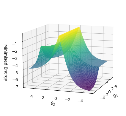
The image is a 3D surface plot visualizing the relationship between "Minimised Energy" and two variables, theta1 (θ₁) and theta2 (θ₂). The surface is colored based on the energy level, with lower energy values represented by purple/blue and higher energy values represented by yellow/green. The plot shows two distinct minima and a central peak.
### Components/Axes
* **X-axis (θ₁):** Ranges from approximately -5 to 5.
* **Y-axis (θ₂):** Ranges from approximately -5 to 5.
* **Z-axis (Minimised Energy):** Ranges from -7 to -1.
* **Color Gradient:** Represents the magnitude of the "Minimised Energy," with purple/blue indicating lower values and yellow/green indicating higher values.
### Detailed Analysis
The surface plot exhibits the following key features:
* **Two Minima:** There are two distinct low-energy regions (purple/blue) located symmetrically with respect to the θ₂ axis. One is located at approximately θ₁ = -4, θ₂ = 4, and the other at θ₁ = -4, θ₂ = -4. The energy at these minima is approximately -7.
* **Central Peak:** A high-energy region (yellow/green) is located near θ₁ = 0, θ₂ = 0. The energy at this peak is approximately -1.
* **Symmetry:** The surface appears to be roughly symmetrical with respect to the θ₂ axis.
* **Slopes:** The surface slopes steeply upwards from the minima towards the central peak.
### Key Observations
* The global minima of the "Minimised Energy" occur at two distinct points in the θ₁-θ₂ space.
* The energy landscape is characterized by steep gradients, suggesting a strong dependence of the energy on the values of θ₁ and θ₂.
* The symmetry of the plot suggests that the energy function might have some inherent symmetry properties.
### Interpretation
The 3D surface plot visualizes an energy landscape where the "Minimised Energy" depends on two parameters, θ₁ and θ₂. The presence of two distinct minima suggests that there are two stable configurations or solutions for the system being modeled. The central peak represents an unstable configuration or a barrier between the two stable states. The steep slopes indicate that small changes in θ₁ or θ₂ can lead to significant changes in the energy. This type of plot is commonly used in optimization problems to visualize the objective function and identify potential solutions.