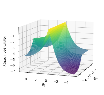
## 3D Surface Plot: Minimised Energy Landscape ### Overview The image depicts a 3D surface plot visualizing a mathematical function's energy landscape. The plot features a color gradient from purple (lowest energy) to yellow (highest energy), with a grid overlay and labeled axes. The surface exhibits multiple peaks, troughs, and saddle points, suggesting a complex optimization problem or physical system. ### Components/Axes - **X-axis (θ₂)**: Ranges from -4 to 4, labeled with integer markers at -4, -2, 0, 2, 4. - **Y-axis (θ₁)**: Ranges from -4 to 4, labeled with integer markers at -4, -2, 0, 2, 4. - **Z-axis (Minimised Energy)**: Ranges from -7 to -1, with markers at -1, -2, -3, -4, -5, -6, -7. - **Grid**: Fine grid lines span all three axes, with darker lines at axis intersections. - **Color Gradient**: Smooth transition from purple (low energy) to yellow (high energy), with no explicit legend but implied by color intensity. ### Detailed Analysis 1. **Peaks**: - **Highest Peak**: Located at approximately (θ₂=0, θ₁=2), with energy ≈ -1 (yellow region). - **Secondary Peak**: Near (θ₂=2, θ₁=0), energy ≈ -2 (green-yellow transition). 2. **Troughs**: - **Deepest Trough**: At (θ₂=-4, θ₁=-4), energy ≈ -7 (dark purple). - **Secondary Trough**: Near (θ₂=4, θ₁=4), energy ≈ -6 (dark purple). 3. **Saddle Point**: - Located at (θ₂=0, θ₁=0), energy ≈ -3 (green region), acting as a critical point between peaks and troughs. 4. **Symmetry**: - The plot exhibits approximate symmetry about θ₂=0, with mirrored energy distributions in the θ₁ direction. ### Key Observations - The energy landscape is non-convex, with multiple local minima and maxima. - The deepest energy minimum (-7) occurs at the extreme corner (-4, -4), while the shallowest (-1) is near the origin. - The saddle point at (0,0) suggests a transition zone between high and low energy regions. - Energy values decrease monotonically from yellow to purple, with no abrupt discontinuities. ### Interpretation This plot likely represents a potential energy surface or cost function in an optimization problem. The saddle point at (0,0) indicates a critical point where the gradient vanishes, which could correspond to an unstable equilibrium in physics or a local extremum in optimization. The asymmetry in peak heights and trough depths suggests the function is not radially symmetric, possibly reflecting constraints or biases in the system. The extreme trough at (-4,-4) implies the function penalizes large negative inputs more severely, which might be relevant for boundary-condition analysis. The absence of a legend necessitates relying on the colorbar's implicit mapping, though the exact numerical-to-color conversion cannot be verified without additional data.