## Chart: Shannon and Bayesian Surprise
### Overview
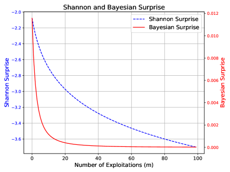
The image is a line chart comparing Shannon Surprise and Bayesian Surprise as a function of the number of exploitations. The chart has two y-axes, one for each type of surprise. The x-axis represents the number of exploitations.
### Components/Axes
* **Title:** Shannon and Bayesian Surprise
* **X-axis:** Number of Exploitations (m), ranging from 0 to 100 in increments of 20.
* **Left Y-axis:** Shannon Surprise, ranging from -3.6 to -2.0 in increments of 0.2.
* **Right Y-axis:** Bayesian Surprise, ranging from 0.000 to 0.012 in increments of 0.002.
* **Legend:** Located at the top-right of the chart.
* Shannon Surprise (blue dashed line)
* Bayesian Surprise (red solid line)
### Detailed Analysis
* **Shannon Surprise (blue dashed line):**
* Trend: Decreases as the number of exploitations increases.
* At 0 exploitations, the Shannon Surprise is approximately -2.1.
* At 20 exploitations, the Shannon Surprise is approximately -3.1.
* At 40 exploitations, the Shannon Surprise is approximately -3.3.
* At 60 exploitations, the Shannon Surprise is approximately -3.45.
* At 80 exploitations, the Shannon Surprise is approximately -3.55.
* At 100 exploitations, the Shannon Surprise is approximately -3.65.
* **Bayesian Surprise (red solid line):**
* Trend: Decreases rapidly initially and then plateaus as the number of exploitations increases.
* At 0 exploitations, the Bayesian Surprise is approximately 0.0115.
* At 20 exploitations, the Bayesian Surprise is approximately 0.0003.
* At 40 exploitations, the Bayesian Surprise is approximately 0.0001.
* At 60 exploitations, the Bayesian Surprise is approximately 0.00005.
* At 80 exploitations, the Bayesian Surprise is approximately 0.00002.
* At 100 exploitations, the Bayesian Surprise is approximately 0.00001.
### Key Observations
* Both Shannon Surprise and Bayesian Surprise decrease as the number of exploitations increases.
* Bayesian Surprise decreases much more rapidly than Shannon Surprise, especially in the initial stages of exploitation.
* Bayesian Surprise approaches zero as the number of exploitations increases, while Shannon Surprise approaches a negative value.
### Interpretation
The chart illustrates how surprise, as measured by Shannon Surprise and Bayesian Surprise, changes with the number of exploitations. The rapid decrease in Bayesian Surprise suggests that the model quickly learns and becomes less surprised by new data as it is exploited. The slower decrease in Shannon Surprise indicates that there is still some uncertainty or information gain even after many exploitations. The difference in the rate of decrease and the final values suggests that the two measures of surprise capture different aspects of the learning process. Bayesian Surprise seems to be more sensitive to initial learning, while Shannon Surprise reflects a more persistent level of uncertainty.