\n
## Line Chart: Shannon and Bayesian Surprise
### Overview
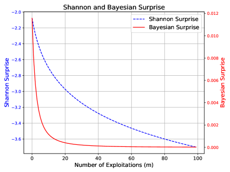
The image presents a line chart comparing Shannon Surprise and Bayesian Surprise as a function of the Number of Exploitations (m). The chart displays two curves, one representing Shannon Surprise and the other Bayesian Surprise, both decreasing as the number of exploitations increases. A secondary y-axis on the right side of the chart displays the scale for Bayesian Surprise.
### Components/Axes
* **Title:** "Shannon and Bayesian Surprise" - positioned at the top-center of the chart.
* **X-axis:** "Number of Exploitations (m)" - ranging from approximately 0 to 100, with tick marks at intervals of 20.
* **Y-axis (left):** "Shannon Surprise" - ranging from approximately -2.0 to -3.5, with tick marks at intervals of 0.2.
* **Y-axis (right):** "Bayesian Surprise" - ranging from approximately 0.000 to 0.012, with tick marks at intervals of 0.002.
* **Legend:** Located in the top-right corner of the chart.
* "Shannon Surprise" - represented by a dashed blue line.
* "Bayesian Surprise" - represented by a solid red line.
* **Gridlines:** Present throughout the chart, aiding in value estimation.
### Detailed Analysis
**Shannon Surprise (Blue Dashed Line):**
The Shannon Surprise line starts at approximately -2.1 at m=0 and decreases gradually, approaching approximately -3.5 at m=100. The line exhibits a steep initial decline, then flattens out as the number of exploitations increases.
* m = 0: Shannon Surprise ≈ -2.1
* m = 20: Shannon Surprise ≈ -2.8
* m = 40: Shannon Surprise ≈ -3.0
* m = 60: Shannon Surprise ≈ -3.2
* m = 80: Shannon Surprise ≈ -3.3
* m = 100: Shannon Surprise ≈ -3.5
**Bayesian Surprise (Red Solid Line):**
The Bayesian Surprise line starts at approximately 0.011 at m=0 and decreases rapidly, approaching 0.000 at m=100. The decline is much steeper than that of the Shannon Surprise line, especially in the initial range.
* m = 0: Bayesian Surprise ≈ 0.011
* m = 20: Bayesian Surprise ≈ 0.002
* m = 40: Bayesian Surprise ≈ 0.001
* m = 60: Bayesian Surprise ≈ 0.0005
* m = 80: Bayesian Surprise ≈ 0.0002
* m = 100: Bayesian Surprise ≈ 0.000
### Key Observations
* Both Shannon and Bayesian Surprise decrease with an increasing number of exploitations.
* Bayesian Surprise decreases much more rapidly than Shannon Surprise.
* Bayesian Surprise approaches zero much faster than Shannon Surprise.
* The initial drop in Bayesian Surprise is very significant, indicating a large change in surprise with the first few exploitations.
### Interpretation
The chart illustrates the concept of diminishing returns in terms of information gain from observing exploitations. Initially, each exploitation provides a significant amount of new information (high surprise), as reflected by the steep decline in Bayesian Surprise. However, as the number of exploitations increases, the information gained from each additional exploitation diminishes (lower surprise).
Shannon Surprise, while also decreasing, does so at a slower rate, suggesting that it captures a different aspect of information content. The difference between the two curves highlights the impact of prior beliefs (Bayesian Surprise) on how information is perceived. Bayesian Surprise incorporates prior knowledge, leading to a more rapid reduction in surprise as evidence accumulates.
The fact that Bayesian Surprise approaches zero suggests that, with enough exploitations, the event becomes highly predictable, and the surprise associated with it vanishes. This could be interpreted as a system reaching a state of equilibrium or complete understanding. The chart demonstrates the utility of Bayesian methods in modeling information gain and predicting event likelihoods.