## Line Chart: Validation Loss vs. Computational Cost (FLOPs) for Different Model Sizes
### Overview
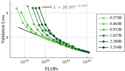
The image is a line chart plotting **Validation Loss** against computational cost, measured in **FLOPs** (Floating Point Operations), for six different neural network model sizes. The chart demonstrates the scaling relationship between model size, computational budget, and performance (loss). All data series show a consistent downward trend, indicating that loss decreases as computational investment increases.
### Components/Axes
* **Chart Type:** Multi-series line chart with markers.
* **X-Axis:**
* **Label:** `FLOPs`
* **Scale:** Logarithmic (base 10).
* **Range:** Approximately `10^19` to `10^22`.
* **Major Ticks:** `10^19`, `10^20`, `10^21`, `10^22`.
* **Y-Axis:**
* **Label:** `Validation Loss`
* **Scale:** Linear.
* **Range:** Approximately 2.5 to 4.5.
* **Major Ticks:** 3, 4.
* **Legend:**
* **Position:** Right side of the chart, vertically centered.
* **Content:** Six entries, each associating a color shade and marker with a model size in billions of parameters (B).
* **Entries (from lightest to darkest green):**
1. `0.275B` (Lightest green, circle marker)
2. `0.464B`
3. `0.932B`
4. `1.627B`
5. `2.280B`
6. `3.354B` (Darkest green, circle marker)
* **Annotation:**
* **Position:** Top-center of the chart area.
* **Content:** A mathematical equation: `L = 26.287^{-0.047}`. This appears to be a fitted power-law curve describing the general trend of loss (`L`) scaling with some underlying variable (likely related to model size or data, though not explicitly stated on the axes).
### Detailed Analysis
Each data series is represented by a line connecting circular markers, with each line corresponding to a specific model size from the legend.
**Trend Verification:** All six lines exhibit a clear, monotonic **downward slope** from left to right. This visually confirms that for every model size, increasing the computational budget (FLOPs) leads to a reduction in validation loss.
**Data Point Approximation (Key Observations from Plot):**
* **Starting Points (Low FLOPs ~10^19 - 10^20):** The lines are vertically separated. The smallest model (`0.275B`, lightest green) starts at the lowest loss (≈3.3 at ~2x10^19 FLOPs), while the largest model (`3.354B`, darkest green) starts at the highest loss (≈4.3 at ~10^20 FLOPs). This indicates that at very low compute budgets, smaller models are more efficient.
* **Convergence (High FLOPs >10^21):** As FLOPs increase, the lines converge. By `10^22` FLOPs, all models achieve a validation loss in a narrow band between approximately 2.6 and 2.8. The lines for the largest models (`2.280B`, `3.354B`) cross over and ultimately achieve slightly lower final loss than the smallest models at the highest compute point shown.
* **Slope:** The rate of loss decrease (slope) appears steeper for the larger models in the mid-range of FLOPs (`10^20` to `10^21`), suggesting they benefit more dramatically from additional compute in that regime.
### Key Observations
1. **Universal Scaling Law:** The consistent, parallel-ish downward trend across all model sizes suggests a fundamental scaling relationship between compute and performance.
2. **Crossover Point:** There is a crossover in efficiency. Smaller models are better at very low compute, but larger models become superior as the compute budget increases beyond approximately `5x10^20` to `10^21` FLOPs.
3. **Diminishing Returns:** The curves flatten as they move to the right, illustrating the principle of diminishing returns—each additional order of magnitude in FLOPs yields a smaller absolute reduction in loss.
4. **Power-Law Fit:** The annotated equation `L = 26.287^{-0.047}` is a power-law function. It likely represents a fitted model for the loss scaling, where the negative exponent (`-0.047`) quantifies the rate of decay. The base (`26.287`) is a scaling constant.
### Interpretation
This chart is a classic visualization of **neural scaling laws**, a critical concept in modern AI research. It demonstrates that model performance (validation loss) improves predictably as a power-law function of the computational resources (FLOPs) invested in training.
The data suggests that to achieve state-of-the-art performance (lowest loss), one must train larger models with more data using a larger compute budget. The convergence of the lines implies that given sufficient compute, model size becomes less of a differentiating factor for final performance, but larger models can reach a given loss threshold with fewer training steps (or less data) once they enter their efficient regime.
The crossover phenomenon is particularly insightful for resource allocation. It argues against using a one-size-fits-all model: for applications with strict limits on training compute, a smaller model is optimal. For applications where maximum performance is the goal and compute is less constrained, investing in a larger model is necessary. The chart provides the empirical basis for making such strategic decisions in AI development.