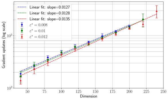
## Scatter Plot with Linear Fits: Gradient Updates vs. Dimension
### Overview
The image is a technical scatter plot with error bars and overlaid linear regression lines. It displays the relationship between the dimension of a system (x-axis) and the number of gradient updates required (y-axis, on a logarithmic scale) for three different values of a parameter denoted as ε* (epsilon star). The plot suggests a power-law or exponential relationship, as the log-scale y-axis versus linear x-axis yields approximately straight lines.
### Components/Axes
* **Chart Type:** Scatter plot with error bars and linear fit lines.
* **X-Axis:**
* **Label:** "Dimension"
* **Scale:** Linear, ranging from approximately 40 to 250.
* **Major Ticks:** 50, 75, 100, 125, 150, 175, 200, 225, 250.
* **Y-Axis:**
* **Label:** "Gradient updates (log scale)"
* **Scale:** Logarithmic (base 10). The visible major ticks are at 10² (100) and 10³ (1000).
* **Legend (Located in the top-left corner of the plot area):**
* **Blue dashed line:** "Linear fit: slope=0.0127"
* **Green dashed line:** "Linear fit: slope=0.0128"
* **Red dashed line:** "Linear fit: slope=0.0135"
* **Blue circle marker with error bar:** "ε* = 0.008"
* **Green square marker with error bar:** "ε* = 0.01"
* **Red triangle marker with error bar:** "ε* = 0.012"
* **Data Series:** Three distinct series, each represented by a specific color/marker combination and accompanied by a linear fit line of the same color.
### Detailed Analysis
**Trend Verification:** All three data series show a clear, consistent upward trend. As the Dimension increases, the number of Gradient updates increases. On this semi-log plot, the trends are approximately linear, indicating an exponential relationship between Gradient updates and Dimension.
**Data Points & Linear Fits (Approximate Values):**
The data points are plotted at discrete Dimension values. The following table reconstructs the approximate y-values (Gradient updates) read from the log-scale axis for each series. The error bars indicate the uncertainty or variance in the measurement.
| Dimension | ε* = 0.008 (Blue Circle) | ε* = 0.01 (Green Square) | ε* = 0.012 (Red Triangle) |
| :--- | :--- | :--- | :--- |
| **~45** | ~150 (Error bar: ~120-180) | ~140 (Error bar: ~110-170) | ~130 (Error bar: ~100-160) |
| **~60** | ~220 (Error bar: ~190-250) | ~200 (Error bar: ~170-230) | ~180 (Error bar: ~150-210) |
| **~80** | ~320 (Error bar: ~280-360) | ~290 (Error bar: ~250-330) | ~260 (Error bar: ~220-300) |
| **~100** | ~450 (Error bar: ~400-500) | ~410 (Error bar: ~360-460) | ~370 (Error bar: ~320-420) |
| **~120** | ~620 (Error bar: ~560-680) | ~570 (Error bar: ~510-630) | ~520 (Error bar: ~460-580) |
| **~140** | ~850 (Error bar: ~780-920) | ~780 (Error bar: ~710-850) | ~710 (Error bar: ~640-780) |
| **~160** | ~1150 (Error bar: ~1050-1250) | ~1050 (Error bar: ~950-1150) | ~960 (Error bar: ~860-1060) |
| **~180** | ~1500 (Error bar: ~1350-1650) | ~1380 (Error bar: ~1230-1530) | ~1250 (Error bar: ~1100-1400) |
| **~200** | ~1950 (Error bar: ~1750-2150) | ~1780 (Error bar: ~1580-1980) | ~1600 (Error bar: ~1400-1800) |
| **~220** | N/A | ~2250 (Error bar: ~2000-2500) | ~2050 (Error bar: ~1800-2300) |
| **~240** | N/A | N/A | ~2600 (Error bar: ~2300-2900) |
**Linear Fit Slopes:**
* Blue (ε* = 0.008): slope = 0.0127
* Green (ε* = 0.01): slope = 0.0128
* Red (ε* = 0.012): slope = 0.0135
### Key Observations
1. **Consistent Linear Scaling:** The primary observation is the strong linear relationship on the semi-log plot for all three series. This indicates that the number of gradient updates grows exponentially with the dimension.
2. **Slope Dependence on ε*:** The slope of the linear fit increases slightly with the value of ε*. The series for ε* = 0.012 (red) has the steepest slope (0.0135), while the slopes for ε* = 0.008 (blue) and ε* = 0.01 (green) are nearly identical (0.0127 vs. 0.0128).
3. **Increasing Variance:** The vertical spread of the error bars appears to increase with Dimension for all series, suggesting that the variance or uncertainty in the number of gradient updates grows as the problem size (dimension) increases.
4. **Data Range:** The blue series (ε* = 0.008) has data points only up to Dimension ~200, while the red series (ε* = 0.012) extends to Dimension ~240. This may indicate experimental limits or convergence behavior.
### Interpretation
This chart demonstrates a fundamental scaling law in an optimization or machine learning context. The "Gradient updates" likely represent the computational cost or training time required for an algorithm to converge. The "Dimension" represents the size or complexity of the model or problem.
The key finding is that this cost scales **exponentially with dimension**, as evidenced by the linear trend on a log-linear plot. This is a significant result, implying that doubling the model dimension more than doubles the required training effort.
The parameter ε* appears to be a tolerance or step-size parameter. The data suggests that a **larger ε* (0.012) leads to a slightly faster increase in cost with dimension** (steeper slope) compared to smaller values. However, at any given dimension, the absolute number of updates is lower for larger ε* (the red points are consistently below the blue and green points). This presents a trade-off: a larger ε* may yield faster initial progress (fewer updates at low dimensions) but becomes relatively less efficient as the problem scales up.
The increasing error bars with dimension highlight that for larger, more complex problems, the performance of the algorithm becomes less predictable, with a wider range of possible outcomes for the number of updates required. This chart would be critical for researchers or engineers to predict computational budgets and choose appropriate hyperparameters (ε*) when scaling up their models.