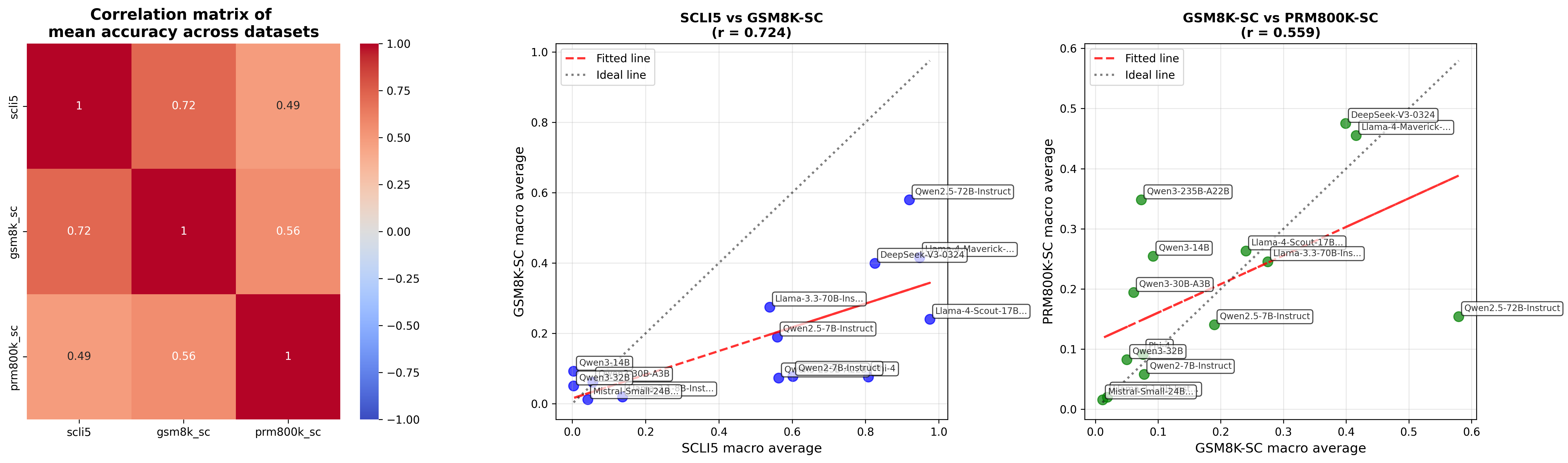
## Chart Type: Multi-Panel Data Analysis ### Overview The image presents a multi-panel data analysis consisting of a correlation matrix and two scatter plots. The correlation matrix displays the mean accuracy correlations between three datasets: scli5, gsm8k_sc, and prm800k_sc. The scatter plots compare the macro averages of these datasets, with fitted lines and ideal lines overlaid to visualize the relationships. ### Components/Axes **Panel 1: Correlation Matrix** * **Title:** Correlation matrix of mean accuracy across datasets * **X-axis Labels:** scli5, gsm8k_sc, prm800k_sc * **Y-axis Labels:** scli5, gsm8k_sc, prm800k_sc * **Color Scale:** Ranges from blue (-1.00) to red (1.00), with white representing 0.00. * **Values:** Displayed within each cell of the matrix. **Panel 2: Scatter Plot 1** * **Title:** SCLI5 vs GSM8K-SC (r = 0.724) * **X-axis Label:** SCLI5 macro average * Scale: 0.0 to 1.0, incrementing by 0.2 * **Y-axis Label:** GSM8K-SC macro average * Scale: 0.0 to 1.0, incrementing by 0.2 * **Data Points:** Blue circles, each labeled with a model name. * **Fitted Line:** Red dashed line. * **Ideal Line:** Gray dotted line. * **Legend (Top-Left):** * Fitted line: Red dashed line * Ideal line: Gray dotted line **Panel 3: Scatter Plot 2** * **Title:** GSM8K-SC vs PRM800K-SC (r = 0.559) * **X-axis Label:** GSM8K-SC macro average * Scale: 0.0 to 0.6, incrementing by 0.1 * **Y-axis Label:** PRM800K-SC macro average * Scale: 0.0 to 0.6, incrementing by 0.1 * **Data Points:** Green circles, each labeled with a model name. * **Fitted Line:** Red dashed line. * **Ideal Line:** Gray dotted line. * **Legend (Top-Left):** * Fitted line: Red dashed line * Ideal line: Gray dotted line ### Detailed Analysis **Panel 1: Correlation Matrix** | | scli5 | gsm8k_sc | prm800k_sc | | :-------- | :---- | :------- | :---------- | | **scli5** | 1 | 0.72 | 0.49 | | **gsm8k_sc** | 0.72 | 1 | 0.56 | | **prm800k_sc**| 0.49 | 0.56 | 1 | * All diagonal values are 1, indicating perfect correlation of a dataset with itself. * scli5 and gsm8k_sc have a strong positive correlation of 0.72. * scli5 and prm800k_sc have a moderate positive correlation of 0.49. * gsm8k_sc and prm800k_sc have a moderate positive correlation of 0.56. **Panel 2: Scatter Plot 1 (SCLI5 vs GSM8K-SC)** * The fitted line (red dashed) shows a positive correlation between SCLI5 and GSM8K-SC macro averages. * The ideal line (gray dotted) represents a 1:1 correlation. * Data points (blue) are scattered around the fitted line, indicating some variance. * **Llama-3.3-70B-Ins...**: Approximately (0.1, 0.1) * **Qwen3-32B**: Approximately (0.1, 0.1) * **Qwen3-30B-A3B**: Approximately (0.2, 0.1) * **Mistral-Small-24B...**: Approximately (0.2, 0.0) * **Qwen2-7B-Instruct i-4**: Approximately (0.5, 0.1) * **Llama-4-Scout-17B...**: Approximately (0.6, 0.2) * **DeepSeek-V3-0324**: Approximately (0.9, 0.4) * **Llama-4-Maverick-...**: Approximately (0.9, 0.4) * **Qwen2.5-72B-Instruct**: Approximately (1.0, 0.6) * **Qwen2.5-7B-Instruct**: Approximately (0.6, 0.2) **Panel 3: Scatter Plot 2 (GSM8K-SC vs PRM800K-SC)** * The fitted line (red dashed) shows a positive correlation between GSM8K-SC and PRM800K-SC macro averages. * The ideal line (gray dotted) represents a 1:1 correlation. * Data points (green) are scattered around the fitted line, indicating some variance. * **Mistral-Small-24B...**: Approximately (0.0, 0.0) * **Qwen2-7B-Instruct**: Approximately (0.1, 0.0) * **Qwen3-32B**: Approximately (0.1, 0.1) * **Qwen3-30B-A3B**: Approximately (0.1, 0.2) * **Qwen3-14B**: Approximately (0.2, 0.25) * **Qwen3-235B-A22B**: Approximately (0.2, 0.35) * **Llama-4-Scout-17B...**: Approximately (0.3, 0.25) * **Llama-3.3-70B-Ins...**: Approximately (0.3, 0.25) * **DeepSeek-V3-0324**: Approximately (0.1, 0.5) * **Llama-4-Maverick-...**: Approximately (0.1, 0.5) * **Qwen2.5-7B-Instruct**: Approximately (0.6, 0.2) ### Key Observations * The correlation matrix indicates a strong relationship between scli5 and gsm8k_sc datasets. * The scatter plots show positive correlations between the datasets, but with noticeable variance around the fitted lines. * The 'r' values (0.724 and 0.559) indicate the strength of the linear correlation, with SCLI5 vs GSM8K-SC having a stronger correlation than GSM8K-SC vs PRM800K-SC. * The data points in the scatter plots represent different models, and their positions indicate their relative performance on the respective datasets. ### Interpretation The data suggests that while there is a positive correlation in mean accuracy across the datasets, the relationships are not perfectly linear. The correlation matrix confirms the inter-relatedness of the datasets, while the scatter plots provide a more granular view of model performance across different dataset pairings. The variance around the fitted lines in the scatter plots indicates that model performance is not consistent across all datasets, and some models may perform better on certain datasets than others. The 'r' values quantify the strength of these relationships, with a higher 'r' value indicating a stronger linear association.

## Scatter Plots & Correlation Matrix: Model Performance Across Datasets ### Overview The image presents a correlation matrix alongside two scatter plots. The correlation matrix visualizes the pairwise correlations between mean accuracy scores across three datasets: SCLIS, GSM8K-SC, and PRMBOOK-SC. The scatter plots compare the performance of different models on pairs of these datasets, with fitted lines and an "ideal line" for reference. ### Components/Axes **Correlation Matrix:** * **Title:** "Correlation matrix of mean accuracy across datasets" * **Labels:** SCLIS, GSM8K-SC, PRMBOOK-SC (along both axes) * **Color Scale:** Ranges from -1.00 (dark blue) to 1.00 (dark red), representing negative to positive correlation. Values are displayed within the matrix cells. **Scatter Plot 1 (SCLIS vs GSM8K-SC):** * **Title:** "SCLIS vs GSM8K-SC (r = 0.724)" * **X-axis:** SCLIS macro average (scale from approximately 0.0 to 1.0) * **Y-axis:** GSM8K-SC macro average (scale from approximately 0.0 to 1.0) * **Lines:** * Fitted line (red, dashed) * Ideal line (green, dotted) * **Data Points:** Labeled with model names (e.g., "Owen2.5-7B-instruct", "DeepSeek-4-3224") **Scatter Plot 2 (GSM8K-SC vs PRMBOOK-SC):** * **Title:** "GSM8K-SC vs PRMBOOK-SC (r = 0.559)" * **X-axis:** GSM8K-SC macro average (scale from approximately 0.0 to 0.6) * **Y-axis:** PRMBOOK-SC macro average (scale from approximately 0.0 to 0.6) * **Lines:** * Fitted line (red, dashed) * Ideal line (green, dotted) * **Data Points:** Labeled with model names (e.g., "Owen2.5-3B", "DeepSeek-4-3224") ### Detailed Analysis or Content Details **Correlation Matrix:** * SCLIS vs GSM8K-SC: 0.72 * SCLIS vs PRMBOOK-SC: 0.49 * GSM8K-SC vs PRMBOOK-SC: 0.56 **Scatter Plot 1 (SCLIS vs GSM8K-SC):** The fitted line slopes upward, indicating a positive correlation. The ideal line is a 45-degree line. * DeepSeek-4-3224: (approximately 0.95, 0.85) * Llama-4-Maverick: (approximately 0.90, 0.75) * Owen2.5-72B-instruct: (approximately 0.85, 0.65) * Llama-4-Scout-17B-ins: (approximately 0.75, 0.55) * Owen2.5-7B-instruct: (approximately 0.70, 0.45) * Owen2.3-32B: (approximately 0.60, 0.35) * Mistral-Small-7B-ins: (approximately 0.50, 0.25) **Scatter Plot 2 (GSM8K-SC vs PRMBOOK-SC):** The fitted line also slopes upward, indicating a positive correlation, but less strong than the first scatter plot. * DeepSeek-4-3224: (approximately 0.55, 0.50) * Llama-4-Maverick: (approximately 0.50, 0.40) * Owen2.5-3B: (approximately 0.40, 0.15) * Owen2.5-72B-instruct: (approximately 0.35, 0.25) * Llama-4-Scout-17B-ins: (approximately 0.30, 0.20) * Owen2.3-32B: (approximately 0.25, 0.10) * Mistral-Small-7B-ins: (approximately 0.20, 0.05) ### Key Observations * The correlation between SCLIS and GSM8K-SC is the strongest (0.72), suggesting that models performing well on one dataset tend to perform well on the other. * The correlation between GSM8K-SC and PRMBOOK-SC is moderate (0.56). * DeepSeek-4-3224 consistently shows high performance across all datasets. * Mistral-Small-7B-ins consistently shows lower performance across all datasets. * The scatter plots show that the fitted lines do not perfectly align with the ideal line, indicating that performance on one dataset does not perfectly predict performance on the other. ### Interpretation The data suggests that there is a degree of transferability in model performance across these datasets, but it is not perfect. Models that excel in one area (e.g., SCLIS) generally perform well in related areas (e.g., GSM8K-SC), but there are exceptions. The correlation matrix quantifies this relationship, while the scatter plots provide a more granular view of individual model performance. The "ideal line" in the scatter plots represents perfect correlation – if a model's performance on the x-axis perfectly predicted its performance on the y-axis, all data points would fall on this line. The deviation from this line indicates the presence of factors beyond the correlation between the two datasets that influence model performance. The consistent high performance of DeepSeek-4-3224 and lower performance of Mistral-Small-7B-ins suggest that model architecture and/or training data play a significant role in determining performance on these tasks. The differences in the slopes of the fitted lines in the two scatter plots indicate that the relationship between GSM8K-SC and PRMBOOK-SC is different than the relationship between SCLIS and GSM8K-SC. This could be due to differences in the nature of the tasks or the data distributions within each dataset.

\n ## Correlation Matrix and Scatter Plots: Model Performance Analysis ### Overview The image contains three distinct charts arranged horizontally. From left to right: a correlation matrix heatmap, a scatter plot comparing SCLI5 vs GSM8K-SC performance, and a scatter plot comparing GSM8K-SC vs PRM800K-SC performance. The overall theme is analyzing the correlation between mean accuracy scores of various language models across three different evaluation datasets. ### Components/Axes **Chart 1 (Left): Correlation Matrix** * **Title:** "Correlation matrix of mean accuracy across datasets" * **Axes Labels (Y-axis, top to bottom):** `scli5`, `gsm8k_sc`, `prm800k_sc` * **Axes Labels (X-axis, left to right):** `scli5`, `gsm8k_sc`, `prm800k_sc` * **Color Bar Legend (Right side):** A vertical gradient bar ranging from blue (-1.00) to red (1.00), with tick marks at -1.00, -0.75, -0.50, -0.25, 0.00, 0.25, 0.50, 0.75, 1.00. **Chart 2 (Middle): Scatter Plot** * **Title:** "SCLI5 vs GSM8K-SC (r = 0.724)" * **X-axis:** "SCLI5 macro average" (Scale: 0.0 to 1.0) * **Y-axis:** "GSM8K-SC macro average" (Scale: 0.0 to 1.0) * **Legend (Top-left):** Contains two entries: "Fitted line" (red dashed line) and "Ideal line" (gray dotted line). * **Data Points:** Blue circles, each labeled with a model name. **Chart 3 (Right): Scatter Plot** * **Title:** "GSM8K-SC vs PRM800K-SC (r = 0.559)" * **X-axis:** "GSM8K-SC macro average" (Scale: 0.0 to 0.6) * **Y-axis:** "PRM800K-SC macro average" (Scale: 0.0 to 0.6) * **Legend (Top-left):** Contains two entries: "Fitted line" (red dashed line) and "Ideal line" (gray dotted line). * **Data Points:** Green circles, each labeled with a model name. ### Detailed Analysis **Chart 1: Correlation Matrix** The heatmap displays Pearson correlation coefficients between the mean accuracy scores on three datasets. * **Diagonal (Self-correlation):** All values are `1` (dark red), as expected. * **Off-diagonal Values:** * `scli5` vs `gsm8k_sc`: **0.72** (medium orange-red) * `scli5` vs `prm800k_sc`: **0.49** (light orange) * `gsm8k_sc` vs `prm800k_sc`: **0.56** (medium orange) * **Interpretation:** The strongest correlation (0.72) is between SCLI5 and GSM8K-SC. The weakest correlation (0.49) is between SCLI5 and PRM800K-SC. **Chart 2: SCLI5 vs GSM8K-SC Scatter Plot** * **Trend:** The data points show a clear positive linear trend. The red "Fitted line" slopes upward from left to right, confirming the positive correlation (r=0.724). Most points lie below the gray "Ideal line" (y=x), indicating that models generally score higher on SCLI5 than on GSM8K-SC. * **Data Points (Approximate Coordinates - X:SCLI5, Y:GSM8K-SC):** * `Qwen2.5-72B-Instruct`: (~0.95, ~0.58) - Highest on both axes. * `Llama-4-Maverick-...`: (~0.90, ~0.40) * `DeepSeek-V3-0324`: (~0.85, ~0.40) * `Llama-3.3-70B-Ins...`: (~0.60, ~0.28) * `Qwen2.5-7B-Instruct`: (~0.55, ~0.19) * `Llama-4-Scout-17B...`: (~0.95, ~0.24) - Notable outlier, high SCLI5 but lower GSM8K-SC. * `Qwen2-7B-Instruct`: (~0.60, ~0.08) * `Qwen3-14B`: (~0.05, ~0.09) * `Qwen3-30B-A3B`: (~0.15, ~0.05) * `Qwen3-32B`: (~0.05, ~0.05) * `Mistral-Small-24B...`: (~0.05, ~0.01) **Chart 3: GSM8K-SC vs PRM800K-SC Scatter Plot** * **Trend:** The data points show a moderate positive linear trend. The red "Fitted line" slopes upward, confirming the correlation (r=0.559). The spread of points around the fitted line is wider than in the middle chart, indicating a noisier relationship. Most points are below the "Ideal line." * **Data Points (Approximate Coordinates - X:GSM8K-SC, Y:PRM800K-SC):** * `DeepSeek-V3-0324`: (~0.40, ~0.48) - Highest on both axes. * `Llama-4-Maverick-...`: (~0.40, ~0.46) * `Qwen3-235B-A22B`: (~0.08, ~0.35) - Notable outlier, very low GSM8K-SC but high PRM800K-SC. * `Qwen3-14B`: (~0.10, ~0.26) * `Llama-4-Scout-17B...`: (~0.25, ~0.26) * `Llama-3.3-70B-Ins...`: (~0.28, ~0.25) * `Qwen3-30B-A3B`: (~0.05, ~0.19) * `Qwen2.5-7B-Instruct`: (~0.19, ~0.14) * `Qwen2.5-72B-Instruct`: (~0.58, ~0.15) - Notable outlier, highest GSM8K-SC but relatively low PRM800K-SC. * `Qwen3-32B`: (~0.08, ~0.08) * `Qwen2-7B-Instruct`: (~0.10, ~0.06) * `Mistral-Small-24B...`: (~0.02, ~0.02) ### Key Observations 1. **Strongest Link:** Performance on SCLI5 and GSM8K-SC is most strongly correlated (r=0.724). 2. **General Underperformance:** In both scatter plots, the majority of models fall below the "Ideal line" (y=x), suggesting they achieve lower macro-average scores on the second dataset (GSM8K-SC or PRM800K-SC) compared to the first (SCLI5 or GSM8K-SC). 3. **Significant Outliers:** * `Llama-4-Scout-17B...` in the middle chart: High SCLI5 score but disproportionately lower GSM8K-SC score. * `Qwen3-235B-A22B` in the right chart: Very low GSM8K-SC score but a high PRM800K-SC score. * `Qwen2.5-72B-Instruct` in the right chart: The highest GSM8K-SC score but a relatively low PRM800K-SC score, breaking the general trend. 4. **Model Clustering:** Lower-performing models (e.g., `Mistral-Small-24B...`, `Qwen3-32B`) cluster near the origin (0,0) in both scatter plots. ### Interpretation The data suggests that the evaluation datasets (SCLI5, GSM8K-SC, PRM800K-SC) measure related but distinct capabilities of language models. The strong correlation between SCLI5 and GSM8K-SC indicates these two benchmarks may be testing similar underlying skills (potentially related to mathematical or logical reasoning, given the "GSM" in the name). The weaker correlation with PRM800K-SC implies it assesses a different dimension of model performance. The consistent pattern of models scoring lower on the second dataset in each pair could indicate that GSM8K-SC and PRM800K-SC are more difficult than SCLI5 and GSM8K-SC, respectively, for this set of models. The notable outliers are crucial: they represent models with specialized strengths or weaknesses. For example, `Qwen3-235B-A22B`'s performance profile suggests it may be uniquely optimized for the tasks in PRM800K-SC while lacking in GSM8K-SC skills. Conversely, `Qwen2.5-72B-Instruct` excels at GSM8K-SC but does not transfer that advantage to PRM800K-SC to the same degree as other top models. This analysis highlights that model evaluation is multi-faceted, and a single aggregate score can mask significant performance variations across different task types.

## Heatmap: Correlation matrix of mean accuracy across datasets ### Overview A 3x3 correlation matrix visualizing relationships between three datasets: scli5, gsm8k_sc, and prm800k_sc. Values range from -1 to 1, with darker red indicating stronger positive correlation. ### Components/Axes - **Rows/Columns**: - Top row: scli5 - Middle row: gsm8k_sc - Bottom row: prm800k_sc - **Color Scale**: - Blue (-1.0) to Red (+1.0) - White (0.0) as midpoint - **Values**: - Diagonal: All 1.0 (perfect self-correlation) - Off-diagonal: - scli5-gsm8k_sc: 0.72 - scli5-prm800k_sc: 0.49 - gsm8k_sc-prm800k_sc: 0.56 ### Detailed Analysis - **scli5**: - Strongest correlation with gsm8k_sc (0.72) - Moderate correlation with prm800k_sc (0.49) - **gsm8k_sc**: - Moderate correlation with prm800k_sc (0.56) - **prm800k_sc**: - Weakest overall correlation (0.49 with scli5) ### Key Observations - All datasets show positive correlations - scli5 and gsm8k_sc share the strongest relationship - prm800k_sc demonstrates weaker but still positive relationships ### Interpretation The matrix reveals that scli5 and gsm8k_sc are most closely related in terms of mean accuracy performance across datasets. prm800k_sc shows more divergent behavior, suggesting different underlying characteristics or performance patterns compared to the other two datasets. --- ## Scatter Plot: SCLI5 vs GSM8K-SC (r = 0.724) ### Overview Scatter plot comparing SCLI5 and GSM8K-SC macro averages with fitted and ideal trend lines. Points labeled with model names. ### Components/Axes - **X-axis**: SCLI5 macro average (0.0-1.0) - **Y-axis**: GSM8K-SC macro average (0.0-1.0) - **Legend**: - Dashed red: Fitted line - Dotted gray: Ideal line (y=x) ### Detailed Analysis - **Trend**: - Fitted line (r=0.724) shows strong positive correlation - Points generally cluster near the ideal line - **Data Points**: - **Bottom-left cluster** (0.0-0.2 SCLI5, 0.0-0.2 GSM8K): - Mistral-Small-24B-Instruct-v1.0 - Qwen3-32B - Qwen3-30B-A3B - **Middle cluster** (0.3-0.6 SCLI5, 0.2-0.4 GSM8K): - Qwen2.5-7B-Instruct - Qwen2.5-7B-Instruct-i4 - Qwen3-14B - **Top-right cluster** (0.7-1.0 SCLI5, 0.4-0.8 GSM8K): - Qwen2.5-72B-Instruct - DeepSeek-V3-0324 - Llama-3-70B-Instruct-v1.0 ### Key Observations - High-performing models (top-right) show strong alignment between SCLI5 and GSM8K-SC - Lower-performing models cluster in the bottom-left - Fitted line closely follows the ideal line, indicating linear relationship ### Interpretation The strong correlation (r=0.724) suggests that performance on SCLI5 strongly predicts performance on GSM8K-SC. The clustering of models indicates distinct performance tiers, with high-performing models showing consistent excellence across both benchmarks. --- ## Scatter Plot: GSM8K-SC vs PRM800K-SC (r = 0.559) ### Overview Scatter plot comparing GSM8K-SC and PRM800K-SC macro averages with fitted and ideal trend lines. Points labeled with model names. ### Components/Axes - **X-axis**: GSM8K-SC macro average (0.0-0.6) - **Y-axis**: PRM800K-SC macro average (0.0-0.6) - **Legend**: - Dashed red: Fitted line - Dotted gray: Ideal line (y=x) ### Detailed Analysis - **Trend**: - Fitted line (r=0.559) shows moderate positive correlation - Points show more dispersion than previous plot - **Data Points**: - **Bottom-left cluster** (0.0-0.2 GSM8K, 0.0-0.2 PRM800K): - Mistral-Small-24B-Instruct-v1.0 - Qwen3-32B - Qwen2.5-7B-Instruct - **Middle cluster** (0.2-0.4 GSM8K, 0.1-0.3 PRM800K): - Qwen3-14B - Llama-3-70B-Instruct-v1.0 - **Top-right cluster** (0.4-0.6 GSM8K, 0.3-0.6 PRM800K): - DeepSeek-V3-0324 - Llama-4-Maverick-17B-Instruct - Qwen2.5-72B-Instruct ### Key Observations - Weaker correlation (r=0.559) compared to SCLI5-GSM8K relationship - More dispersed data points indicate less consistent relationships - High-performing models show better alignment with the fitted line ### Interpretation The moderate correlation suggests that while there's some relationship between GSM8K-SC and PRM800K-SC performance, it's less consistent than the SCLI5-GSM8K relationship. The dispersion of points indicates that models may perform differently across these benchmarks, suggesting varying strengths in different reasoning domains. --- ## Cross-Plot Analysis 1. **Consistency**: - SCLI5-GSM8K shows strongest correlation (r=0.724) - GSM8K-PRM800K shows weakest correlation (r=0.559) 2. **Model Performance**: - Qwen2.5-72B-Instruct consistently performs best across all benchmarks - Mistral-Small-24B-Instruct-v1.0 consistently performs worst 3. **Trend Lines**: - Fitted lines in both scatter plots closely follow ideal lines, suggesting linear relationships - steeper slope in SCLI5-GSM8K plot indicates stronger relationship ## Conclusion The correlation matrix and scatter plots reveal distinct performance patterns across different reasoning benchmarks. The strong SCLI5-GSM8K relationship suggests shared characteristics in these benchmarks, while the weaker GSM8K-PRM800K relationship indicates more divergent performance characteristics. Model performance tiers are clearly distinguishable, with high-performing models showing consistent excellence across all benchmarks.