## Line Graph: Model Accuracy vs. Compute (exaFLOP)
### Overview
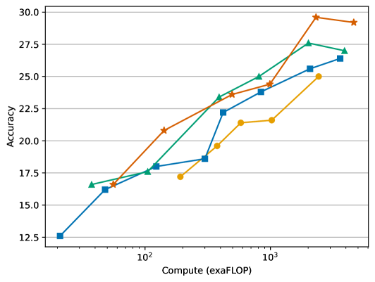
The graph illustrates the relationship between computational resources (exaFLOP) and model accuracy for four distinct models (A, B, C, D). Accuracy improves with increased compute, but the rate of improvement varies significantly across models. The x-axis uses a logarithmic scale (10² to 10³ exaFLOP), while the y-axis is linear (12.5–30.0 accuracy).
### Components/Axes
- **X-axis (Compute)**: Logarithmic scale (10² to 10³ exaFLOP), labeled "Compute (exaFLOP)".
- **Y-axis (Accuracy)**: Linear scale (12.5–30.0), labeled "Accuracy".
- **Legend**: Located in the top-right corner, mapping colors to models:
- **Orange (★)**: Model A
- **Green (▲)**: Model B
- **Blue (■)**: Model C
- **Yellow (●)**: Model D
### Detailed Analysis
1. **Model A (Orange ★)**:
- **Trend**: Sharp initial increase in accuracy, followed by a plateau.
- **Data Points**:
- ~16.5 exaFLOP → ~17.5 accuracy
- ~21 exaFLOP → ~21 accuracy
- ~1000 exaFLOP → ~29.5 accuracy
- **Key Insight**: Achieves near-peak accuracy (~29.5) at the highest compute but shows diminishing returns after ~21 exaFLOP.
2. **Model B (Green ▲)**:
- **Trend**: Steady, linear increase in accuracy.
- **Data Points**:
- ~17 exaFLOP → ~17 accuracy
- ~100 exaFLOP → ~22.5 accuracy
- ~1000 exaFLOP → ~27.5 accuracy
- **Key Insight**: Maintains consistent improvement but lags behind Model A at lower compute levels.
3. **Model C (Blue ■)**:
- **Trend**: Slow initial growth, followed by accelerated improvement.
- **Data Points**:
- ~18 exaFLOP → ~18 accuracy
- ~100 exaFLOP → ~22 accuracy
- ~1000 exaFLOP → ~26 accuracy
- **Key Insight**: Outperforms Model B at higher compute but underperforms at lower compute.
4. **Model D (Yellow ●)**:
- **Trend**: Gradual increase with a slight dip mid-range.
- **Data Points**:
- ~19 exaFLOP → ~19 accuracy
- ~100 exaFLOP → ~21 accuracy
- ~1000 exaFLOP → ~25 accuracy
- **Key Insight**: Least efficient model, requiring the most compute for marginal gains.
### Key Observations
- **Efficiency Variance**: Model A achieves the highest accuracy (~29.5) with the least compute (~1000 exaFLOP), while Model D requires similar compute for ~25 accuracy.
- **Diminishing Returns**: Model A plateaus near its peak accuracy, suggesting architectural limits.
- **Compute Thresholds**: All models show significant accuracy jumps between 10² and 10³ exaFLOP, but Model A’s early gains are most pronounced.
### Interpretation
The data highlights a trade-off between computational cost and accuracy. Model A demonstrates superior efficiency, achieving near-optimal performance with minimal resources. In contrast, Model D’s gradual improvement suggests suboptimal design or training. The logarithmic x-axis emphasizes that even modest compute increases (e.g., 10x) yield disproportionate accuracy gains, particularly for Models A and B. This underscores the importance of architectural optimization over brute-force scaling. The plateau in Model A’s performance raises questions about hardware/software co-design limits, while Model D’s inefficiency may indicate overfitting or poor resource utilization.