## Line Chart: Shannon and Bayesian Surprises ### Overview The image is a line chart comparing Shannon Surprise and Bayesian Surprise over a number of explorations. The x-axis represents the "Number of Explorations (m)" ranging from 0 to 100. The left y-axis represents "Shannon Surprise" ranging from 0 to 8, while the right y-axis represents "Bayesian Surprise" ranging from 0.0 to 20.0. The Shannon Surprise is represented by a dashed blue line, and the Bayesian Surprise is represented by a solid red line. ### Components/Axes * **Title:** Shannon and Bayesian Surprises * **X-axis:** * Label: Number of Explorations (m) * Range: 0 to 100 * Ticks: 0, 20, 40, 60, 80, 100 * **Left Y-axis:** * Label: Shannon Surprise * Range: 0 to 8 * Ticks: 0, 1, 2, 3, 4, 5, 6, 7, 8 * **Right Y-axis:** * Label: Bayesian Surprise * Range: 0.0 to 20.0 * Ticks: 0.0, 2.5, 5.0, 7.5, 10.0, 12.5, 15.0, 17.5, 20.0 * **Legend:** Located in the top-right corner. * Shannon Surprise: Dashed blue line * Bayesian Surprise: Solid red line ### Detailed Analysis * **Shannon Surprise (Dashed Blue Line):** * Trend: Highly variable, with several peaks and troughs, generally decreasing after around exploration 40. * Approximate Data Points: * Exploration 0: ~2.5 * Exploration 10: ~3.5 * Exploration 20: ~2.0 * Exploration 30: ~3.5 * Exploration 40: ~5.0 * Exploration 50: ~2.0 * Exploration 60: ~1.0 * Exploration 70: ~0.5 * Exploration 80: ~2.5 * Exploration 90: ~1.0 * Exploration 100: ~0.2 * **Bayesian Surprise (Solid Red Line):** * Trend: Generally low with occasional spikes, decreasing to near zero after exploration 60. * Approximate Data Points: * Exploration 0: ~4.0 * Exploration 5: ~3.0 * Exploration 10: ~1.0 * Exploration 20: ~3.0 * Exploration 30: ~1.0 * Exploration 40: ~2.0 * Exploration 50: ~3.0 * Exploration 60: ~0.1 * Exploration 70: ~0.1 * Exploration 80: ~0.1 * Exploration 90: ~0.1 * Exploration 100: ~0.1 ### Key Observations * The Shannon Surprise exhibits more frequent and larger fluctuations compared to the Bayesian Surprise. * Both Shannon and Bayesian Surprise tend to decrease as the number of explorations increases, especially after exploration 60. * The Bayesian Surprise is generally lower than the Shannon Surprise, except for the initial explorations. ### Interpretation The chart illustrates how Shannon and Bayesian Surprises change with an increasing number of explorations. The Shannon Surprise, which measures information gain, shows high variability, suggesting that the agent frequently encounters unexpected information. The Bayesian Surprise, which measures the change in belief, is generally lower and decreases more consistently, indicating that the agent's beliefs stabilize as it explores the environment. The decrease in both surprises over time suggests that the agent is learning and becoming more familiar with the environment, leading to fewer unexpected events and smaller belief updates. The spikes in Bayesian Surprise indicate specific instances where the agent's beliefs were significantly altered, possibly due to encountering critical new information.

\n ## Line Chart: Shannon and Bayesian Surprises ### Overview The image presents a line chart comparing Shannon Surprise and Bayesian Surprise over a number of explorations (m). The chart displays two distinct lines representing each surprise metric, plotted against the number of explorations, ranging from 0 to 100. The y-axis for Shannon Surprise is on the left, ranging from 0 to 8, while the y-axis for Bayesian Surprise is on the right, ranging from 0 to 20. ### Components/Axes * **Title:** "Shannon and Bayesian Surprises" (centered at the top) * **X-axis:** "Number of Explorations (m)" (bottom, ranging from 0 to 100) * **Left Y-axis:** "Shannon Surprise" (ranging from 0 to 8) * **Right Y-axis:** "Bayesian Surprise" (ranging from 0 to 20) * **Legend:** Located in the top-right corner. * "Shannon Surprise" - represented by a dashed blue line. * "Bayesian Surprise" - represented by a solid red line. ### Detailed Analysis **Bayesian Surprise (Red Line):** The red line representing Bayesian Surprise starts at approximately 1.8 at m=0, rises to a peak of around 2.2 at m=2, then rapidly declines to near 0 by m=10. It remains very close to 0 for the majority of the exploration range (m=10 to m=90), with minor fluctuations. At m=90, it rises to approximately 1.5 and then falls back to near 0 at m=100. The trend is generally decreasing, with a sharp initial drop and then a sustained low level. **Shannon Surprise (Blue Dashed Line):** The blue dashed line representing Shannon Surprise exhibits a much more volatile pattern. It starts at approximately 0.5 at m=0, rises to a peak of around 3.5 at m=4, then falls to approximately 1.5 at m=8. It continues to fluctuate significantly throughout the exploration range, with multiple peaks and valleys. Notable peaks occur around m=12 (approximately 3.0), m=20 (approximately 3.5), m=30 (approximately 4.0), m=40 (approximately 5.0), m=50 (approximately 3.0), m=60 (approximately 3.5), m=70 (approximately 2.5), and m=80 (approximately 3.0). The line ends at approximately 1.0 at m=100. The trend is highly variable, with no clear overall direction. ### Key Observations * Bayesian Surprise is consistently much lower than Shannon Surprise for most of the exploration range. * Shannon Surprise exhibits significant fluctuations, indicating a high degree of uncertainty or information gain during exploration. * Bayesian Surprise drops rapidly and remains low, suggesting that the initial surprise quickly diminishes as the exploration progresses. * There is a noticeable peak in Shannon Surprise around m=40, which is significantly higher than other peaks. * Both lines show some activity around m=90, but the Bayesian Surprise remains very low. ### Interpretation The chart suggests that the initial explorations provide a significant amount of information (high Shannon Surprise), but this information quickly becomes predictable (low Bayesian Surprise). The sustained low Bayesian Surprise indicates that the exploration process is converging on a relatively stable understanding of the environment. The fluctuations in Shannon Surprise suggest that there are still unexpected events or discoveries occurring throughout the exploration process, even after the initial period of high surprise. The peak at m=40 could represent a particularly informative or surprising event during the exploration. The difference between the two surprise measures highlights the distinction between the raw amount of information gained (Shannon Surprise) and the information that is relevant given prior beliefs (Bayesian Surprise). The chart demonstrates how Bayesian Surprise can filter out irrelevant information, focusing on the unexpected events that truly challenge existing beliefs.

## Line Chart: Shannon and Bayesian Surprises ### Overview This is a dual-axis line chart comparing two metrics, "Shannon Surprise" and "Bayesian Surprise," plotted against the "Number of Explorations (m)." The chart displays how these two measures of surprise or information gain evolve over a sequence of exploratory actions. ### Components/Axes * **Chart Title:** "Shannon and Bayesian Surprises" (centered at the top). * **X-Axis:** * **Label:** "Number of Explorations (m)" * **Scale:** Linear, ranging from 0 to 100 with major tick marks every 20 units (0, 20, 40, 60, 80, 100). * **Primary Y-Axis (Left):** * **Label:** "Shannon Surprise" * **Scale:** Linear, ranging from 0 to 8 with major tick marks every 1 unit. * **Associated Data Series:** Blue dashed line. * **Secondary Y-Axis (Right):** * **Label:** "Bayesian Surprise" * **Scale:** Linear, ranging from 0.0 to 20.0 with major tick marks every 2.5 units. * **Associated Data Series:** Red solid line. * **Legend:** Located in the top-right corner of the plot area. * **Blue dashed line:** "Shannon Surprise" * **Red solid line:** "Bayesian Surprise" * **Grid:** A light gray grid is present, aligned with the major ticks of both the x-axis and the primary (left) y-axis. ### Detailed Analysis **Data Series Trends and Key Points:** 1. **Shannon Surprise (Blue Dashed Line, Left Axis):** * **Trend:** The series exhibits high volatility with frequent, sharp spikes, particularly in the first half of the exploration sequence (m=0 to m=60). The magnitude of the spikes generally decreases as the number of explorations increases. After approximately m=60, the values drop significantly and remain low, with only a few minor spikes. * **Key Data Points (Approximate):** * Initial value at m=0: ~2.8 * Major peaks: * m ≈ 10: ~4.5 * m ≈ 35: ~4.8 (highest peak) * m ≈ 45: ~3.7 * m ≈ 85: ~2.8 * Values after m=60 are predominantly below 1.0, often near 0. 2. **Bayesian Surprise (Red Solid Line, Right Axis):** * **Trend:** This series also shows spiky behavior, with peaks that are temporally correlated with the peaks in Shannon Surprise. However, its overall magnitude (on its own scale) is lower relative to its axis maximum. The trend shows a more pronounced decline after the initial explorations, approaching and staying near zero from approximately m=60 onward. * **Key Data Points (Approximate):** * Initial value at m=0: ~3.5 * Major peaks (correlated with Shannon peaks): * m ≈ 10: ~5.0 * m ≈ 35: ~4.0 * m ≈ 45: ~3.5 * m ≈ 85: ~3.5 * Values after m=60 are consistently very low, frequently at or near 0.0. **Spatial and Visual Correlation:** The peaks of both lines are closely aligned along the x-axis, indicating that events causing a high Shannon Surprise also cause a high Bayesian Surprise. The red line (Bayesian) appears to have a slightly smoother baseline between spikes compared to the blue line (Shannon). ### Key Observations 1. **Strong Correlation:** The most notable pattern is the tight temporal correlation between spikes in Shannon Surprise and Bayesian Surprise. They rise and fall together. 2. **Diminishing Surprise:** Both metrics show a clear overall trend of diminishing magnitude as the number of explorations (m) increases. The most significant "surprises" occur early in the process. 3. **Phase Transition:** There is a distinct change in behavior around m=60. After this point, both surprise measures become quiescent, suggesting the system or model has largely assimilated the environment or data, leading to few new surprises. 4. **Scale Difference:** While correlated, the absolute values are measured on different scales. A Shannon Surprise of ~4.8 corresponds to a Bayesian Surprise of ~4.0 at m≈35. ### Interpretation This chart likely visualizes the learning or adaptation process of an agent or model in an unknown environment. "Surprise" quantifies the discrepancy between expectation and observation. * **What the data suggests:** The early exploratory phase (m < 60) is characterized by frequent, significant updates to the model's beliefs, as evidenced by high surprise values. Each exploration provides substantial new information. The perfect correlation between the two surprise metrics indicates they are capturing related, though mathematically distinct, aspects of information gain. Shannon Surprise is rooted in information theory (reduction in entropy), while Bayesian Surprise measures the divergence between prior and posterior belief distributions. * **How elements relate:** The x-axis represents time or experience. The dual y-axes allow the comparison of two different quantitative measures of the same conceptual phenomenon ("surprise") on their native scales. The decline in both lines demonstrates the principle of learning: as the agent explores, its predictions become more accurate, and observations become less surprising. * **Notable anomalies/implications:** The near-zero values after m=60 are critical. They imply the learning process has converged or the environment has become predictable. The few late spikes (e.g., at m≈85) could represent rare, novel events or a change in the environment that temporarily reintroduces uncertainty. The chart effectively argues that both Shannon and Bayesian surprise are valid, correlated signals for guiding exploration, with the most informative explorations happening early on.

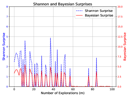
## Line Graph: Shannon and Bayesian Surprises ### Overview The image is a line graph comparing two metrics, "Shannon Surprise" and "Bayesian Surprise," plotted against the "Number of Explorations (m)" on the x-axis. The graph includes two y-axes: the left axis (blue dashed line) represents "Shannon Surprise" (0–8), and the right axis (red solid line) represents "Bayesian Surprise" (0–20). The legend is positioned in the top-right corner, with blue dashed lines for Shannon Surprise and red solid lines for Bayesian Surprise. ### Components/Axes - **Title**: "Shannon and Bayesian Surprises" (centered at the top). - **X-axis**: "Number of Explorations (m)" with a linear scale from 0 to 100. - **Y-axes**: - Left: "Shannon Surprise" (0–8, increments of 1). - Right: "Bayesian Surprise" (0–20, increments of 2.5). - **Legend**: Top-right corner, with: - Blue dashed line: "Shannon Surprise" - Red solid line: "Bayesian Surprise" ### Detailed Analysis - **Shannon Surprise (Blue Dashed Line)**: - Peaks occur at approximately 10m, 20m, 30m, 40m, 50m, 60m, 70m, 80m, and 90m. - Maximum value: ~7.5 (at ~20m and ~40m). - Minimum value: ~0 (at ~0m, ~60m, and ~100m). - Trend: Irregular, with sharp spikes and troughs, suggesting high variability. - **Bayesian Surprise (Red Solid Line)**: - Peaks occur at approximately 10m, 30m, 50m, 70m, and 90m. - Maximum value: ~15 (at ~30m and ~70m). - Minimum value: ~0 (at ~0m, ~60m, and ~100m). - Trend: More consistent peaks compared to Shannon Surprise, with smoother transitions between values. ### Key Observations 1. **Scale Disparity**: The Bayesian Surprise metric operates on a scale 2.5× larger than Shannon Surprise, despite both being labeled as "surprise" measures. 2. **Peak Correlation**: Both metrics share peak positions at ~10m, ~30m, ~50m, ~70m, and ~90m, suggesting a shared underlying pattern in exploration milestones. 3. **Shannon Variability**: Shannon Surprise exhibits more frequent and erratic fluctuations (e.g., ~20m, ~40m, ~80m), while Bayesian Surprise remains relatively stable between peaks. 4. **Axis Independence**: The dual y-axes imply the metrics are not directly comparable in magnitude but may represent different dimensions of "surprise." ### Interpretation The graph illustrates two distinct methods of quantifying "surprise" during exploration. The Shannon Surprise metric (blue) appears more sensitive to short-term fluctuations, with sharp peaks and troughs, possibly reflecting immediate uncertainties or information gains. In contrast, the Bayesian Surprise metric (red) shows broader, more sustained peaks, potentially capturing cumulative or probabilistic surprises over exploration intervals. The shared peak positions suggest that certain exploration milestones (e.g., 10m, 30m) are critical for both metrics, though their magnitudes differ significantly. The scale disparity raises questions about normalization or unit differences between the two methods. This could indicate that Bayesian Surprise is designed to aggregate or smooth data, while Shannon Surprise prioritizes granular, real-time variability. The absence of data beyond 100m explorations may imply a cutoff in the study or a stabilization of surprise metrics at later stages.