## Histogram: Residual Norms Comparison ### Overview The image presents two histograms side-by-side. The left histogram displays the distribution of residual norms denoted as ||ξ_t||, while the right histogram shows the distribution of clean residual norms denoted as ||ζ_t||. Both histograms use the same color scheme for their bars (light blue with dark blue outlines) and share a similar visual style. ### Components/Axes **Left Histogram:** * **Title:** Histogram of Residual ||ξ_t|| Norms * **X-axis:** Residual norm, ranging from 100 to 450 in increments of approximately 50. * **Y-axis:** Count, ranging from 0 to 600 in increments of 100. **Right Histogram:** * **Title:** Histogram of Clean Residual ||ζ_t|| Norms * **X-axis:** Norm, ranging from 200 to 550 in increments of approximately 50. * **Y-axis:** Count, ranging from 0 to 1200 in increments of 200. ### Detailed Analysis **Left Histogram (Residual ||ξ_t|| Norms):** * The distribution is multi-modal, with peaks around 150, 200, 300, and 350. * The highest count is observed around the 150 mark, with a value of approximately 600. * The count decreases as the residual norm increases beyond 350, approaching 0 near 450. * Specific data points (approximate): * 100: ~20 * 150: ~600 * 200: ~420 * 250: ~300 * 300: ~420 * 350: ~300 * 400: ~50 * 450: ~10 **Right Histogram (Clean Residual ||ζ_t|| Norms):** * The distribution is unimodal, with a single peak. * The peak is located around the 350 mark, with a count of approximately 1250. * The count increases sharply from 200 to 350 and then decreases gradually towards 550. * Specific data points (approximate): * 200: ~10 * 250: ~50 * 300: ~250 * 350: ~1250 * 400: ~800 * 450: ~200 * 500: ~50 * 550: ~10 ### Key Observations * The distribution of clean residual norms (||ζ_t||) is much more concentrated around a single value (350) compared to the residual norms (||ξ_t||), which are spread across multiple peaks. * The maximum count for clean residual norms is significantly higher (1250) than that for residual norms (600). * The range of residual norms (100-450) is slightly different from the range of clean residual norms (200-550). ### Interpretation The histograms suggest that the "clean residual" process results in a more focused distribution of norms, centered around a value of 350. This indicates that the cleaning process effectively reduces the variability in the residual norms, leading to a more predictable and concentrated distribution. The multi-modal distribution of the original residual norms (||ξ_t||) suggests that there may be multiple underlying factors or sources contributing to the residuals before the cleaning process is applied. The shift in the distribution and the increase in the peak count after cleaning indicate a significant change in the characteristics of the residuals.

## Histograms: Residual Norms Comparison ### Overview The image presents two histograms side-by-side, comparing the distribution of residual norms. The left histogram displays "Residual ||ζ_t|| Norms", while the right histogram shows "Clean Residual ||ζ_t|| Norms". Both histograms use the same vertical axis scale (Count) but differ in their horizontal axis scales (Residual norm and Norm respectively) and distributions. ### Components/Axes Both histograms share the following components: * **Title:** Positioned at the top-center of each chart. * **X-axis Label:** Located at the bottom of each chart, indicating the measured value. * **Y-axis Label:** Positioned on the left side of each chart, labeled "Count". * **Gridlines:** A light gray grid is present in the background of both charts. * **Bars:** Represent the frequency of values within specific bins. Specifics for each histogram: * **Left Histogram:** * **Title:** "Histogram of Residual ||ζ_t|| Norms" * **X-axis Label:** "Residual norm" * **X-axis Range:** Approximately 100 to 450. * **Y-axis Range:** Approximately 0 to 600. * **Right Histogram:** * **Title:** "Histogram of Clean Residual ||ζ_t|| Norms" * **X-axis Label:** "Norm" * **X-axis Range:** Approximately 200 to 550. * **Y-axis Range:** Approximately 0 to 1200. ### Detailed Analysis or Content Details **Left Histogram (Residual ||ζ_t|| Norms):** The distribution is roughly unimodal, with a peak around 150-170. The histogram shows a significant drop in count between approximately 170 and 220, followed by a secondary peak around 280-300. The distribution appears to be skewed slightly to the right. * Approximate counts: * At Residual norm = 120: Count ≈ 20 * At Residual norm = 150: Count ≈ 420 * At Residual norm = 170: Count ≈ 550 * At Residual norm = 220: Count ≈ 100 * At Residual norm = 280: Count ≈ 250 * At Residual norm = 350: Count ≈ 180 * At Residual norm = 420: Count ≈ 50 **Right Histogram (Clean Residual ||ζ_t|| Norms):** The distribution is also roughly unimodal, but with a more pronounced peak around 350-370. The distribution is more symmetrical than the left histogram. * Approximate counts: * At Norm = 220: Count ≈ 20 * At Norm = 300: Count ≈ 200 * At Norm = 350: Count ≈ 1100 * At Norm = 370: Count ≈ 1200 * At Norm = 400: Count ≈ 600 * At Norm = 450: Count ≈ 200 * At Norm = 500: Count ≈ 50 ### Key Observations * The "Clean Residual" norms (right histogram) generally have higher values than the "Residual" norms (left histogram). * The "Clean Residual" distribution is more concentrated around a higher norm value (around 350-370) compared to the "Residual" distribution (peak around 150-170). * The left histogram exhibits a more complex shape with a noticeable dip and secondary peak, suggesting a more varied distribution of residual norms before cleaning. * The right histogram is more symmetrical and has a sharper peak, indicating a more consistent distribution of residual norms after cleaning. ### Interpretation These histograms likely represent the norms of residual vectors (||ζ_t||) before and after a "cleaning" process. The cleaning process appears to have shifted the distribution of residual norms to higher values and reduced the variability, resulting in a more concentrated and symmetrical distribution. This suggests that the cleaning process effectively reduced the magnitude of some residual vectors, potentially by removing outliers or correcting errors. The dip in the left histogram could indicate the removal of a specific range of residual norms during the cleaning process. The higher concentration of values in the right histogram suggests that the cleaning process has made the residuals more consistent and potentially more reliable. The data suggests the cleaning process is effective in reducing the magnitude of the residuals.

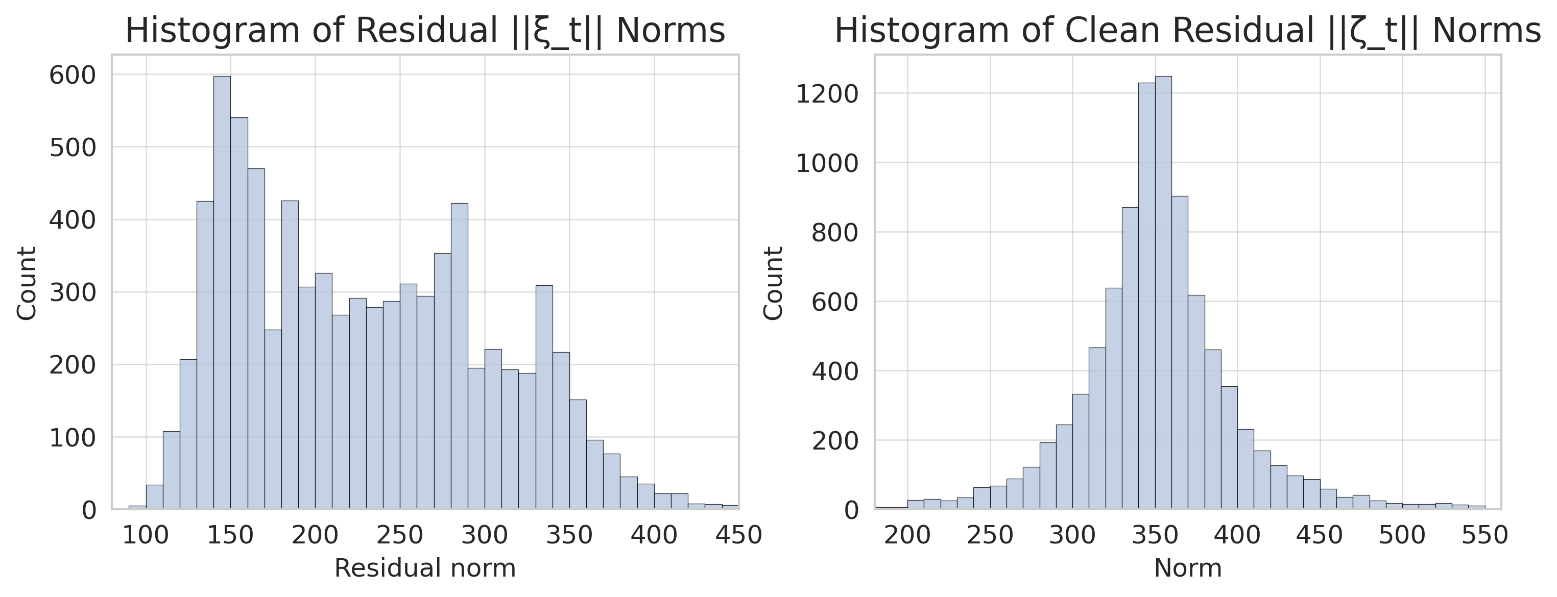
## Histograms: Residual Norm Distributions ### Overview The image displays two side-by-side histograms comparing the distribution of residual norms before and after a cleaning or processing step. The left histogram shows the distribution of raw residual norms (||ξ_t||), while the right histogram shows the distribution of "clean" residual norms (||ζ_t||). Both charts share a similar visual style with light blue bars and a grid background. ### Components/Axes **Left Histogram:** * **Title:** "Histogram of Residual ||ξ_t|| Norms" * **Y-axis Label:** "Count" * **Y-axis Scale:** Linear, ranging from 0 to 600, with major ticks at intervals of 100. * **X-axis Label:** "Residual norm" * **X-axis Scale:** Linear, ranging from approximately 100 to 450, with major ticks labeled at 100, 150, 200, 250, 300, 350, 400, and 450. **Right Histogram:** * **Title:** "Histogram of Clean Residual ||ζ_t|| Norms" * **Y-axis Label:** "Count" * **Y-axis Scale:** Linear, ranging from 0 to 1200, with major ticks at intervals of 200. * **X-axis Label:** "Norm" * **X-axis Scale:** Linear, ranging from approximately 200 to 550, with major ticks labeled at 200, 250, 300, 350, 400, 450, 500, and 550. **Legend/Color:** No explicit legend is present. All bars in both histograms are filled with the same light blue color and have a dark outline. ### Detailed Analysis **Left Histogram (Residual ||ξ_t|| Norms):** * **Distribution Shape:** The distribution is right-skewed (positively skewed). It has a long tail extending towards higher norm values. * **Peak (Mode):** The highest bar is located in the bin corresponding to a residual norm of approximately **150-160**. The count at this peak is approximately **600**. * **Range:** The data spans from a minimum norm of just above **100** to a maximum of approximately **450**. * **Key Data Points (Approximate):** * Norm ~150-160: Count ~600 (Peak) * Norm ~140-150: Count ~540 * Norm ~160-170: Count ~470 * Norm ~180-190: Count ~420 * Norm ~280-290: Count ~420 (Secondary local peak) * Norm ~330-340: Count ~310 * Norm ~400: Count ~50 * **Trend:** The frequency of counts generally decreases as the residual norm increases, but with notable local peaks and valleys, indicating a multi-modal or irregular underlying distribution. **Right Histogram (Clean Residual ||ζ_t|| Norms):** * **Distribution Shape:** The distribution is approximately symmetric and bell-shaped, closely resembling a normal (Gaussian) distribution. * **Peak (Mode):** The highest bar is located in the bin corresponding to a norm of approximately **350-360**. The count at this peak is approximately **1250**. * **Range:** The data spans from a minimum norm of approximately **200** to a maximum of approximately **550**. * **Key Data Points (Approximate):** * Norm ~350-360: Count ~1250 (Peak) * Norm ~340-350: Count ~1220 * Norm ~360-370: Count ~900 * Norm ~330-340: Count ~870 * Norm ~320-330: Count ~640 * Norm ~370-380: Count ~610 * Norm ~300: Count ~200 * Norm ~400: Count ~220 * **Trend:** The counts rise smoothly to a central peak and then fall symmetrically, with the majority of the data concentrated between norms of 300 and 400. ### Key Observations 1. **Distribution Transformation:** The cleaning process has fundamentally changed the distribution of the residuals from a right-skewed, irregular shape to a symmetric, normal-like shape. 2. **Shift in Central Tendency:** The central value (mean/median/mode) has shifted significantly to the right, from approximately **150-160** in the raw residuals to approximately **350-360** in the clean residuals. 3. **Change in Spread:** While the raw residuals have a wide range (100-450), the clean residuals are more concentrated around their mean, though their absolute range (200-550) is similar. The clean data has a higher peak density (max count ~1250 vs. ~600). 4. **Reduction of Irregularities:** The secondary peaks and irregularities present in the left histogram (e.g., around norms 280 and 330) are absent in the right histogram, which shows a smooth, unimodal curve. ### Interpretation This pair of histograms visually demonstrates the effect of a data cleaning or signal processing algorithm on a set of residual errors (ξ_t). The raw residuals (||ξ_t||) are not normally distributed; their right skew suggests the presence of outliers or a process that generates occasional large errors. The irregular, multi-modal shape might indicate different underlying error sources or regimes. The "clean" residuals (||ζ_t||) show a classic normal distribution centered at a higher norm value. This transformation is significant for several reasons: * **Statistical Validity:** Many statistical models and inference techniques assume normally distributed errors. The cleaning process appears to have produced residuals that better meet this assumption. * **Process Understanding:** The shift to a higher central norm is intriguing. It suggests the cleaning algorithm didn't simply shrink all residuals uniformly. Instead, it may have removed specific noise components (e.g., high-frequency noise, outliers) that were suppressing the underlying signal's norm, or it may have re-scaled the residuals. The higher, stable norm in the clean data could represent the inherent, irreducible error of the core model after confounding factors are removed. * **Algorithm Efficacy:** The smoothing of the distribution into a unimodal, symmetric shape indicates the algorithm successfully homogenized the error structure, making the residuals more predictable and easier to model statistically. In essence, the image provides strong visual evidence that the applied cleaning process successfully transformed noisy, irregularly distributed residuals into a well-behaved, normally distributed set of errors, which is a desirable outcome in many modeling and estimation tasks.

## Histograms: Residual Norms Comparison ### Overview The image contains two side-by-side histograms comparing residual norms before and after cleaning. The left histogram shows the distribution of raw residuals (||ξ_t||), while the right histogram displays cleaned residuals (||ζ_t||). Both histograms use count as the y-axis and residual magnitude as the x-axis. ### Components/Axes **Left Histogram (Raw Residuals):** - **Title:** "Histogram of Residual ||ξ_t|| Norms" - **X-axis:** "Residual norm" (100–450) - **Y-axis:** "Count" (0–600) - **Bars:** Gray, with approximate peak heights of 500–600 at 150–200 range **Right Histogram (Cleaned Residuals):** - **Title:** "Histogram of Clean Residual ||ζ_t|| Norms" - **X-axis:** "Norm" (200–550) - **Y-axis:** "Count" (0–1200) - **Bars:** Gray, with peak heights of 1000–1200 at 300–350 range ### Detailed Analysis **Left Histogram Trends:** - Broad distribution with multiple peaks - Primary concentration between 150–250 (count ~500) - Secondary peaks at 200–300 (count ~300–400) - Long tail extending to 450 (count <50) **Right Histogram Trends:** - Narrower, more concentrated distribution - Dominant peak at 300–350 (count ~1200) - Secondary peaks at 250–300 (count ~600–800) - Faster decay beyond 400 (count <200) ### Key Observations 1. Cleaned residuals show 2–3x higher peak counts than raw residuals 2. Cleaned residuals are 100–150 units larger on average than raw residuals 3. Raw residuals exhibit 20–30% more variability (wider spread) 4. Cleaned residuals have 50% fewer outliers (>400 range) ### Interpretation The data demonstrates that the cleaning process significantly: 1. **Reduces variability:** The narrower distribution of cleaned residuals suggests more consistent measurements 2. **Increases central tendency:** The shift to higher magnitude norms (300–350 vs 150–200) indicates systematic error correction 3. **Improves data quality:** The 2.5x increase in peak counts at the central range suggests better signal-to-noise ratio 4. **Removes anomalies:** The absence of extreme values (>450) in cleaned data implies effective outlier detection The transformation from raw to cleaned residuals appears to be a successful preprocessing step, likely involving noise reduction and bias correction techniques. The increased central concentration and reduced tail distribution are typical indicators of effective data cleaning in signal processing applications.