## Chart Compilation: Model Training and Performance Analysis
### Overview
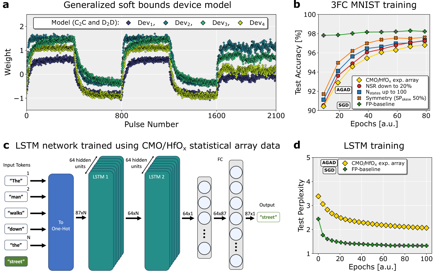
The image presents a compilation of four charts (a, b, c, d) detailing the training and performance of various models, including a generalized soft bounds device model, a 3FC MNIST training model, and an LSTM network. The charts showcase weight distributions, test accuracy, network architecture, and test perplexity.
### Components/Axes
**Chart a: Generalized soft bounds device model**
* **Title:** Generalized soft bounds device model
* **X-axis:** Pulse Number (0 to 2100, approximately)
* **Y-axis:** Weight (-1 to 2, approximately)
* **Data Series:**
* Model (C₂C and D₂D): Dark teal scatter plot.
* Dev₁: Red diamonds.
* Dev₂: Green triangles.
* Dev₃: Blue squares.
* Dev₄: Purple crosses.
**Chart b: 3FC MNIST training**
* **Title:** 3FC MNIST training
* **X-axis:** Epochs [a.u.] (0 to 80, approximately)
* **Y-axis:** Test Accuracy [%] (90 to 100, approximately)
* **Legend (top-left):**
* AGAD: Orange line with diamond markers.
* CMO/HfOₓ exp. array: Red line with circle markers.
* NSR down to 20%: Blue line with square markers.
* Nstates up to 100: Purple line with triangle markers.
* Symmetry (SP skew 50%): Green line with cross markers.
* FP-baseline: Yellow line with plus markers.
**Chart c: LSTM network trained using CMO/HfOₓ statistical array data**
* **Title:** LSTM network trained using CMO/HfOₓ statistical array data
* **Components:** Input Tokens, LSTM 1, LSTM 2, FC (Fully Connected), Output.
* **Input Tokens:** "The", "man", "walks", "down", "the", "street".
* **LSTM Layers:** Two LSTM layers, each with 64 hidden units. Input is 87xN, output is 64xN.
* **FC Layer:** Fully connected layer with 87x87 dimensions.
* **Output:** "street".
**Chart d: LSTM training**
* **Title:** LSTM training
* **X-axis:** Epochs [a.u.] (0 to 100, approximately)
* **Y-axis:** Test Perplexity (1 to 5, approximately)
* **Legend (top-left):**
* AGAD: Orange line with diamond markers.
* CMO/HfOₓ exp. array: Red line with circle markers.
* FP-baseline: Green line with plus markers.
### Detailed Analysis or Content Details
**Chart a:** The teal scatter plot representing the model weights fluctuates around zero, with a generally decreasing trend in amplitude as the pulse number increases. The Dev series (red, green, blue, purple) show relatively stable values, with some fluctuations. Dev₁ is consistently around 98.5, Dev₂ around 97.5, Dev₃ around 96.5, and Dev₄ around 95.5.
**Chart b:** The AGAD line (orange) shows a slight upward trend, starting around 92% and reaching approximately 98.5% accuracy. The CMO/HfOₓ exp. array (red) line starts at approximately 96% and plateaus around 98%. The NSR down to 20% (blue) line shows a similar trend, starting around 92% and reaching approximately 97.5%. The Nstates up to 100 (purple) line starts around 92% and reaches approximately 97%. The Symmetry (SP skew 50%) (green) line starts around 92% and reaches approximately 97.5%. The FP-baseline (yellow) line starts around 92% and reaches approximately 96.5%.
**Chart c:** The diagram illustrates a two-layer LSTM network. Input tokens are converted to one-hot vectors. Each LSTM layer has 64 hidden units. The output layer is a fully connected layer that predicts the next token ("street").
**Chart d:** The AGAD line (orange) shows a decreasing trend in test perplexity, starting around 4.5 and reaching approximately 2.5. The CMO/HfOₓ exp. array (red) line shows a similar decreasing trend, starting around 4.5 and reaching approximately 2. The FP-baseline (green) line shows a decreasing trend, starting around 4.5 and reaching approximately 3.
### Key Observations
* All models in Chart b demonstrate increasing test accuracy with increasing epochs, but the rate of improvement varies.
* The LSTM network in Chart d shows a clear reduction in test perplexity with training, indicating improved language modeling performance.
* The weight distribution in Chart a appears to stabilize over time, suggesting the model is converging.
* The LSTM network architecture in Chart c is relatively simple, consisting of two LSTM layers and a fully connected output layer.
### Interpretation
The data suggests that the models are successfully learning from the training data. The increasing test accuracy in Chart b and decreasing test perplexity in Chart d indicate that the models are improving their ability to generalize to unseen data. The weight distribution in Chart a suggests that the model is converging to a stable state. The LSTM network architecture in Chart c is a standard configuration for language modeling tasks.
The different data series in Chart b (AGAD, CMO/HfOₓ, etc.) represent different training configurations or model architectures. Comparing their performance can provide insights into the effectiveness of different techniques. The fact that all models achieve high accuracy suggests that the MNIST dataset is relatively easy to learn.
The LSTM network in Chart d demonstrates the effectiveness of recurrent neural networks for sequence modeling tasks. The decreasing test perplexity indicates that the model is learning to predict the next token in a sequence with increasing accuracy. The choice of input tokens ("The man walks down the street") suggests that the model is being trained to understand simple sentences.
The overall compilation of charts provides a comprehensive overview of the training and performance of various models, highlighting the strengths and weaknesses of different approaches. The data suggests that the models are performing well, but further analysis may be needed to identify areas for improvement.