\n
## [Line Chart with Annotations]: Comparison of LLMSR and PiT-PO Optimization Performance
### Overview
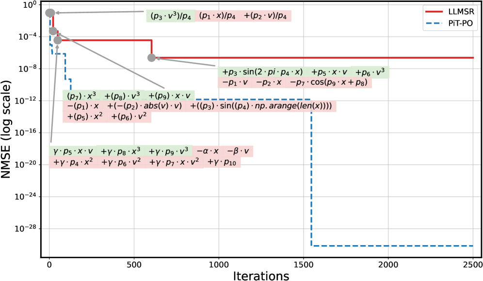
The image is a technical line chart comparing the performance of two optimization methods, **LLMSR** and **PiT-PO**, over a series of iterations. The performance metric is **NMSE (Normalized Mean Squared Error)** plotted on a logarithmic scale. The chart includes detailed mathematical annotations for each method, showing the specific model equations or terms being optimized at different stages. The primary visual narrative is that the **PiT-PO** method (blue dashed line) achieves a significantly lower final error (NMSE) than the **LLMSR** method (red solid line).
### Components/Axes
* **Chart Type:** Line chart with annotations.
* **X-Axis:** Label: **"Iterations"**. Scale: Linear, from 0 to 2500, with major ticks at 0, 500, 1000, 1500, 2000, 2500.
* **Y-Axis:** Label: **"NMSE (log scale)"**. Scale: Logarithmic (base 10), ranging from 10⁰ (1) at the top to 10⁻²⁸ at the bottom. Major ticks are at every power of 100 (10⁰, 10⁻⁴, 10⁻⁸, 10⁻¹², 10⁻¹⁶, 10⁻²⁰, 10⁻²⁴, 10⁻²⁸).
* **Legend:** Located in the **top-right corner**.
* **Red solid line:** Labeled **"LLMSR"**.
* **Blue dashed line:** Labeled **"PiT-PO"**.
* **Annotations:** Mathematical expressions are placed directly on the chart, color-coded and connected to specific points on the lines with arrows or proximity.
* **Green background boxes:** Associated with the **PiT-PO** (blue dashed) line.
* **Pink background boxes:** Associated with the **LLMSR** (red solid) line.
### Detailed Analysis
**1. LLMSR (Red Solid Line) Trend & Data:**
* **Trend:** The line starts at a high NMSE (~10⁰) at iteration 0. It drops very sharply within the first ~100 iterations to approximately 10⁻⁴. It then experiences a second, smaller drop around iteration 600 to about 10⁻⁶. After this point, the line plateaus and remains constant at ~10⁻⁶ until iteration 2500.
* **Annotations (Pink Boxes):**
* **Initial Model (near start):** `(p₃·v³)/p₄ (p₁·x)/p₄ +(p₂·v)/p₄`
* **Model after first drop (near iteration 600):** `+p₃·sin(2·pi·p₄·x) +p₅·x·v +p₆·v³ -p₁·v -p₂·x -p₇·cos(p₉·x + p₈)`
* **Final Plateau Model (spanning iterations ~600-2500):** `(p₇)·x³ +(p₈)·v³ +(p₉)·x·v -(p₁)·x +(-p₂)·abs(v)·v +((p₃)·sin((p₄)·np.arange(len(x)))) +(p₅)·x² +(p₆)·v²`
**2. PiT-PO (Blue Dashed Line) Trend & Data:**
* **Trend:** The line starts at a lower initial NMSE than LLMSR, approximately 10⁻². It shows a stepwise descent. The first major drop occurs within the first ~200 iterations, falling to ~10⁻¹². It then plateaus briefly before a second dramatic drop around iteration 1500, plummeting to an extremely low NMSE of ~10⁻³⁰. It remains at this level until iteration 2500.
* **Annotations (Green Boxes):**
* **Initial/Early Model (near start):** `γ·p₅·x·v +γ·p₈·x³ +γ·p₉·v³ -α·x -β·v +γ·p₄·x² +γ·p₆·v² +γ·p₇·x·v² +γ·p₁₀`
### Key Observations
1. **Performance Gap:** There is a massive performance difference at convergence. PiT-PO's final NMSE (~10⁻³⁰) is approximately **24 orders of magnitude lower** than LLMSR's final NMSE (~10⁻⁶).
2. **Convergence Behavior:** LLMSR converges quickly to a moderate error level and then stagnates. PiT-PO shows a more complex, multi-stage convergence, ultimately reaching a far superior solution.
3. **Model Complexity:** The annotations suggest the models being optimized are nonlinear, involving polynomial terms (x³, v³, x², v²), trigonometric functions (sin, cos), absolute values, and array operations (`np.arange`). The PiT-PO annotation appears simpler in this snapshot, but this may represent only one phase of its optimization.
4. **Visual Grounding:** The color-coding is consistent. All green-highlighted equations are near the blue dashed line. All pink-highlighted equations are near the red solid line. The legend correctly identifies the line styles.
### Interpretation
This chart demonstrates the superior optimization capability of the **PiT-PO** method compared to **LLMSR** for the specific problem being modeled. The problem involves finding parameters (`p₁` through `p₁₀`, `α`, `β`, `γ`) for a complex, nonlinear dynamical system or function involving variables `x` and `v`.
* **What the data suggests:** PiT-PO is not only more effective (reaching a much lower error) but may also employ a more sophisticated or adaptive optimization strategy, as evidenced by its stepwise convergence. The plateau in LLMSR suggests it may have become trapped in a local minimum.
* **Relationship between elements:** The annotations are crucial. They show that the optimization isn't just minimizing a black-box error; it's refining a specific, interpretable mathematical model. The change in the annotated equation for LLMSR around iteration 600 corresponds to its second drop in error, indicating a shift in the model structure or parameter focus during optimization.
* **Notable Anomalies:** The most striking feature is the extreme final precision of PiT-PO (10⁻³⁰). In many practical applications, such a low NMSE is indistinguishable from zero and may indicate the method has found an exact or near-exact analytical solution to the problem. The chart effectively argues for the adoption of PiT-PO over LLMSR for this class of problems.