## Diagram and Chart: Transverse Field Ising Model Simulation and Correlation Analysis
### Overview
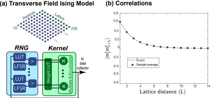
The image is a two-part technical figure. Part (a) is a schematic diagram illustrating the architecture of a simulation for the Transverse Field Ising Model, highlighting its lattice structure and computational kernel. Part (b) is a line graph plotting the spin-spin correlation function against lattice distance, comparing an exact theoretical result with a sample average from the simulation.
### Components/Axes
**Part (a): Transverse Field Ising Model Diagram**
* **Top Section (Lattice Schematic):**
* A 3D-perspective grid of blue dots representing a lattice.
* **Labels:** "Replicas" (pointing along one axis), "Lattice" (pointing along another axis).
* **Numerical Markers:** "10" at the near corner of the replica axis, "250" at the far corner of the lattice axis.
* **Bottom Section (Computational Block Diagram):**
* **Two main colored blocks:**
1. **RNG (Blue Block):** Contains two visible pairs of sub-blocks. Each pair consists of a "LUT" (Look-Up Table) and an "LFSR" (Linear Feedback Shift Register), connected to a comparator symbol (">"). A vertical ellipsis ("...") indicates additional, identical pairs.
2. **Kernel (Green Block):** Contains a vertical "Weight LUT" bar. To its right are multiple "Multiply & Accumulate" units, each depicted as a circle with an "X" (multiplier) connected to a summation symbol ("+"). A vertical ellipsis ("...") indicates multiple such units.
* **Data Flow:** Arrows show connections from the RNG block's comparators to the Kernel's "Weight LUT". The output from the Kernel's "Multiply & Accumulate" units points to the right with the label "to data collector".
**Part (b): Correlations Graph**
* **Title:** "(b) Correlations"
* **Y-axis:**
* **Label:** `<m_i^z m_{i+L}^z>` (This denotes the expectation value of the product of z-component spins at sites separated by distance L).
* **Scale:** Linear, ranging from -0.8 to 0.8 with major ticks at intervals of 0.2.
* **X-axis:**
* **Label:** "Lattice distance (L)"
* **Scale:** Linear, ranging from 0 to 14 with major ticks at every even integer (0, 2, 4, ..., 14).
* **Legend:** Located in the bottom-left quadrant of the plot area.
* **"Exact"**: Represented by a black dashed line (`---`).
* **"Sample average"**: Represented by solid blue circles (`●`).
* **Data Series:**
* The "Exact" series is a smooth, monotonically decreasing dashed curve.
* The "Sample average" series consists of discrete blue data points plotted at integer L values from 1 to 14.
### Detailed Analysis
**Part (a) - Component Flow:**
The diagram describes a computational pipeline. The RNG (Random Number Generator) block, using LUTs and LFSRs, generates random inputs. These are fed into the Kernel block, where they are processed by a Weight LUT and then through parallel Multiply & Accumulate units. The final result is sent to a data collector. The lattice schematic above suggests this kernel operates on a system with 250 lattice sites, possibly across 10 replicas.
**Part (b) - Data Point Extraction & Trend Verification:**
* **Trend:** Both the "Exact" line and the "Sample average" points show a clear, monotonic **downward trend**. The correlation starts at a positive value for L=1 and decays asymptotically towards zero as the lattice distance (L) increases.
* **Approximate Data Points (Sample Average - Blue Dots):**
* L=1: ~0.58
* L=2: ~0.38
* L=3: ~0.22
* L=4: ~0.12
* L=5: ~0.06
* L=6: ~0.03
* L=7: ~0.01
* L=8 to L=14: Values are very close to 0, hovering just above or on the zero line.
* **Cross-Reference:** The blue "Sample average" dots align very closely with the black dashed "Exact" line across the entire range of L, indicating high accuracy of the simulation.
### Key Observations
1. **Strong Agreement:** The simulation's "Sample average" results are in excellent agreement with the "Exact" theoretical curve, validating the computational model depicted in part (a).
2. **Exponential-like Decay:** The correlation function decays rapidly, losing most of its magnitude within the first 4-5 lattice distances.
3. **Long-Range Behavior:** For distances greater than L=7, the correlation is effectively zero, indicating that spins separated by more than ~7 lattice sites are uncorrelated in this model.
4. **Architectural Clarity:** The block diagram in (a) clearly separates the random number generation (RNG) from the core computational kernel, which performs weighted accumulation.
### Interpretation
This figure serves to **validate a hardware or algorithmic implementation** of a Transverse Field Ising Model simulation. Part (a) details the custom computational architecture, emphasizing its use of parallel random number generation (via LUTs/LFSRs) and a dedicated kernel for weighted calculations. Part (b) provides the critical evidence that this implementation works correctly: the measured spin-spin correlations from the simulation ("Sample average") match the known theoretical result ("Exact").
The data demonstrates the fundamental physical property of **short-range order** in the simulated system. The rapid decay of `<m_i^z m_{i+L}^z>` shows that the influence of one spin on another diminishes quickly with distance, a characteristic feature of many statistical mechanical systems at finite temperature or in certain quantum phases. The near-perfect match between simulation and theory suggests the architecture in (a) is a faithful and accurate tool for studying such models.