# Technical Data Extraction: Model Accuracy vs. Generation Budget
## 1. Image Overview
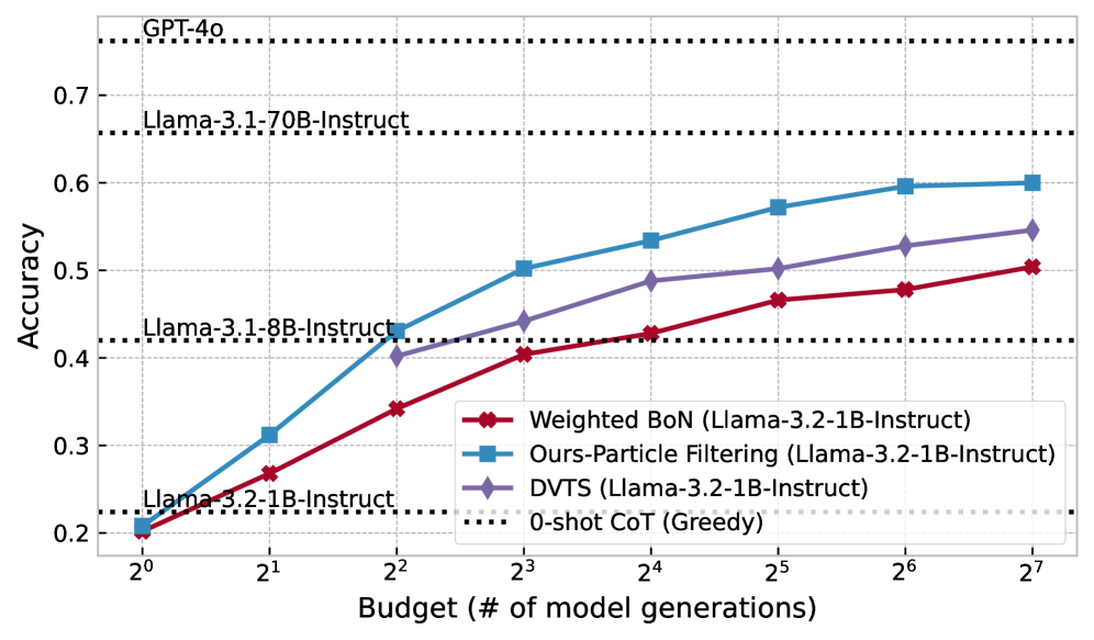
This image is a line graph comparing the performance (Accuracy) of different inference methods applied to the **Llama-3.2-1B-Instruct** model against various baseline models. The performance is measured relative to a computational "Budget," defined as the number of model generations.
## 2. Axis Definitions
* **Y-Axis (Vertical):** Accuracy.
* **Range:** 0.2 to 0.7+ (labeled increments of 0.1).
* **X-Axis (Horizontal):** Budget (# of model generations).
* **Scale:** Logarithmic (base 2).
* **Markers:** $2^0, 2^1, 2^2, 2^3, 2^4, 2^5, 2^6, 2^7$ (representing 1 to 128 generations).
## 3. Baseline Reference Lines (Horizontal Dotted Lines)
These lines represent "0-shot CoT (Greedy)" performance for specific models, acting as static benchmarks.
* **GPT-4o:** Accuracy $\approx$ 0.76
* **Llama-3.1-70B-Instruct:** Accuracy $\approx$ 0.66
* **Llama-3.1-8B-Instruct:** Accuracy $\approx$ 0.42
* **Llama-3.2-1B-Instruct:** Accuracy $\approx$ 0.225
## 4. Legend and Data Series Analysis
The legend is located in the bottom-right quadrant of the chart area.
### Series 1: Ours-Particle Filtering (Llama-3.2-1B-Instruct)
* **Visual Identifier:** Blue line with square markers.
* **Trend:** Steepest upward slope in the early stages ($2^0$ to $2^3$), maintaining the highest accuracy among the 1B model methods across all budget levels.
* **Key Data Points (Approximate):**
* $2^0$: 0.21
* $2^2$: 0.43 (Surpasses Llama-3.1-8B-Instruct baseline)
* $2^7$: 0.60 (Approaching Llama-3.1-70B-Instruct baseline)
### Series 2: DVTS (Llama-3.2-1B-Instruct)
* **Visual Identifier:** Purple line with diamond markers.
* **Trend:** Steady upward slope. Starts at $2^2$ budget. Consistently performs between the Particle Filtering and Weighted BoN methods.
* **Key Data Points (Approximate):**
* $2^2$: 0.40
* $2^4$: 0.49
* $2^7$: 0.55
### Series 3: Weighted BoN (Llama-3.2-1B-Instruct)
* **Visual Identifier:** Red line with diamond markers.
* **Trend:** Upward slope, but the shallowest of the three experimental methods.
* **Key Data Points (Approximate):**
* $2^0$: 0.20
* $2^3$: 0.40
* $2^7$: 0.505
## 5. Summary Table of Extracted Data (Estimated Values)
| Budget ($2^n$) | Weighted BoN (Red) | Ours-Particle Filtering (Blue) | DVTS (Purple) |
| :--- | :--- | :--- | :--- |
| **$2^0$ (1)** | 0.20 | 0.21 | - |
| **$2^1$ (2)** | 0.27 | 0.31 | - |
| **$2^2$ (4)** | 0.34 | 0.43 | 0.40 |
| **$2^3$ (8)** | 0.40 | 0.50 | 0.44 |
| **$2^4$ (16)** | 0.43 | 0.53 | 0.49 |
| **$2^5$ (32)** | 0.47 | 0.57 | 0.50 |
| **$2^6$ (64)** | 0.48 | 0.60 | 0.53 |
| **$2^7$ (128)** | 0.51 | 0.60 | 0.55 |
## 6. Key Findings
1. **Scaling Efficiency:** The "Ours-Particle Filtering" method applied to a 1B model achieves the accuracy of a 0-shot 8B model with a budget of only 4 generations ($2^2$).
2. **Closing the Gap:** With a budget of 128 generations ($2^7$), the 1B model using Particle Filtering reaches ~60% accuracy, significantly narrowing the gap toward the 70B model's 66% baseline.
3. **Method Superiority:** Particle Filtering consistently outperforms both Weighted Best-of-N (BoN) and DVTS across the entire tested budget range.