TECHNICAL ASSET FINGERPRINT
474bc9851d77e75468d99776
Click to view fullscreen
Press ESC or click to close
FOUND IN PAPERS
EXPERT: gemini-3.1-pro-preview VERSION 1
RUNTIME: gemini/gemini-3.1-pro-preview
INTEL_VERIFIED
## Diagram: Code Comparison - LLM vs. LLM + APOLLO
### Overview
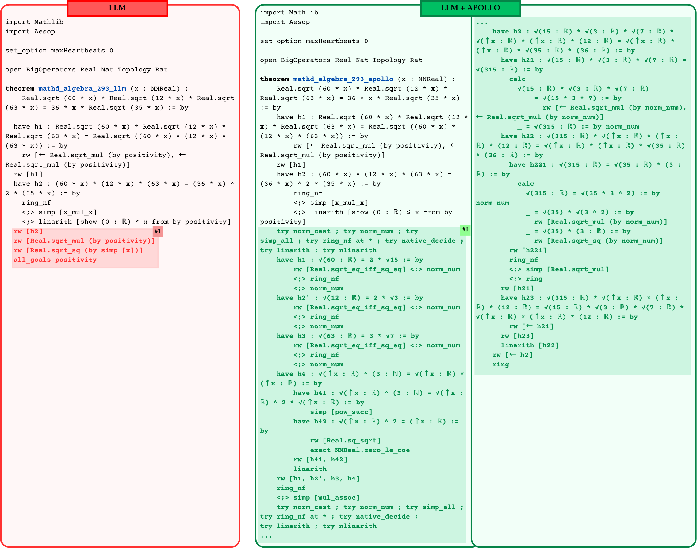
The image displays a side-by-side comparison of two code snippets written in the Lean 4 theorem proving language. The left panel, outlined and headered in red, represents an output generated by a standard "LLM" (Large Language Model). The right panel, outlined and headered in green, represents an output generated by "LLM + APOLLO". Both scripts attempt to prove the same mathematical theorem (`mathd_algebra_293`). The visual design (red vs. green) strongly implies that the left approach fails or is flawed, while the right approach succeeds. Specific lines of code in both panels are highlighted and tagged with "#1" to draw attention to differing methodologies.
### Components/Layout
* **Left Panel (Red):**
* **Header:** "LLM" (White text on a red background, top center).
* **Border:** Solid red line.
* **Content:** A single column of Lean 4 code.
* **Highlight:** A block of code at the bottom is highlighted in light red with a dark red tag labeled `#1` positioned to the right of the first highlighted line.
* **Right Panel (Green):**
* **Header:** "LLM + APOLLO" (White text on a green background, top center).
* **Border:** Solid green line.
* **Content:** Lean 4 code that spans two columns. The code begins in the left half of the green box, reaches the bottom, and continues in a second column on the right half of the green box.
* **Highlight:** A single line of code in the middle of the first column is highlighted in light green with a dark green tag labeled `#1` positioned to the right.
### Content Details
#### Left Panel Transcription (LLM)
```lean
import Mathlib
import Aesop
set_option maxHeartbeats 0
open BigOperators Real Nat Topology Rat
theorem mathd_algebra_293_llm (x : NNReal) :
Real.sqrt (60 * x) * Real.sqrt (12 * x) * Real.sqrt (63 * x) = 36 * x * Real.sqrt (35 * x) := by
have h1 : Real.sqrt (60 * x) * Real.sqrt (12 * x) * Real.sqrt (63 * x) = Real.sqrt ((60 * x) * (12 * x) * (63 * x)) := by
rw [← Real.sqrt_mul (by positivity), ← Real.sqrt_mul (by positivity)]
rw [h1]
have h2 : (60 * x) * (12 * x) * (63 * x) = (36 * x) ^ 2 * (35 * x) := by
ring_nf
<;> simp [x_mul_x]
<;> linarith [show (0 : ℝ) ≤ x from by positivity]
```
*Highlighted Red Section (Tag #1):*
```lean
rw [h2]
rw [Real.sqrt_mul (by positivity)]
rw [Real.sqrt_sq (by simp [x])]
all_goals positivity
```
#### Right Panel Transcription (LLM + APOLLO)
*First Column:*
```lean
import Mathlib
import Aesop
set_option maxHeartbeats 0
open BigOperators Real Nat Topology Rat
theorem mathd_algebra_293_apollo (x : NNReal) :
Real.sqrt (60 * x) * Real.sqrt (12 * x) * Real.sqrt (63 * x) = 36 * x * Real.sqrt (35 * x) := by
have h1 : Real.sqrt (60 * x) * Real.sqrt (12 * x) * Real.sqrt (63 * x) = Real.sqrt ((60 * x) * (12 * x) * (63 * x)) := by
rw [← Real.sqrt_mul (by positivity), ← Real.sqrt_mul (by positivity)]
rw [h1]
have h2 : (60 * x) * (12 * x) * (63 * x) = (36 * x) ^ 2 * (35 * x) := by
ring_nf
<;> simp [x_mul_x]
<;> linarith [show (0 : ℝ) ≤ x from by positivity]
```
*Highlighted Green Section (Tag #1):*
```lean
try norm_cast ; try norm_num ; try simp_all ; try ring_nf at * ; try native_decide ; try linarith ; try nlinarith
```
*First Column (Continued below highlight):*
```lean
have h1 : √(60 : ℝ) = 2 * √15 := by
rw [Real.sqrt_eq_iff_sq_eq] <;> norm_num
<;> ring_nf
<;> norm_num
have h2' : √(12 : ℝ) = 2 * √3 := by
rw [Real.sqrt_eq_iff_sq_eq] <;> norm_num
<;> ring_nf
<;> norm_num
have h3 : √(63 : ℝ) = 3 * √7 := by
rw [Real.sqrt_eq_iff_sq_eq] <;> norm_num
<;> ring_nf
<;> norm_num
have h4 : √(↑x : ℝ) ^ (3 : ℕ) = √(↑x : ℝ) * (↑x : ℝ) := by
have h41 : √(↑x : ℝ) ^ (3 : ℕ) = √(↑x : ℝ) ^ 2 * √(↑x : ℝ) := by
simp [pow_succ]
have h42 : √(↑x : ℝ) ^ 2 = (↑x : ℝ) := by
rw [Real.sq_sqrt]
exact NNReal.zero_le_coe
rw [h41, h42]
linarith
rw [h1, h2', h3, h4]
ring_nf
<;> simp [mul_assoc]
try norm_cast ; try norm_num ; try simp_all ; try ring_nf at * ; try native_decide ; try linarith ; try nlinarith
...
```
*Second Column (Right side of the green panel):*
```lean
...
have h2 : √(15 : ℝ) * √(3 : ℝ) * √(7 : ℝ) * √(↑x : ℝ) * (↑x : ℝ) * (12 : ℝ) = √(↑x : ℝ) * (↑x : ℝ) * √(35 : ℝ) * (36 : ℝ) := by
have h21 : √(15 : ℝ) * √(3 : ℝ) * √(7 : ℝ) = √(315 : ℝ) := by
calc
√(15 : ℝ) * √(3 : ℝ) * √(7 : ℝ)
= √(15 * 3 * 7) := by
rw [← Real.sqrt_mul (by norm_num), ← Real.sqrt_mul (by norm_num)]
_ = √(315 : ℝ) := by norm_num
have h22 : √(315 : ℝ) * √(↑x : ℝ) * (↑x : ℝ) * (12 : ℝ) = √(↑x : ℝ) * (↑x : ℝ) * √(35 : ℝ) * (36 : ℝ) := by
have h221 : √(315 : ℝ) = √(35 : ℝ) * (3 : ℝ) := by
calc
√(315 : ℝ) = √(35 * 3 ^ 2) := by norm_num
_ = √(35) * √(3 ^ 2) := by
rw [Real.sqrt_mul (by norm_num)]
_ = √(35) * (3 : ℝ) := by
rw [Real.sqrt_sq (by norm_num)]
rw [h221]
ring_nf
<;> simp [Real.sqrt_mul]
<;> ring
rw [h21]
have h23 : √(315 : ℝ) * √(↑x : ℝ) * (↑x : ℝ) * (12 : ℝ) = √(15 : ℝ) * √(3 : ℝ) * √(7 : ℝ) * √(↑x : ℝ) * (↑x : ℝ) * (12 : ℝ) := by
rw [← h21]
rw [h23]
linarith [h22]
rw [← h2]
ring
```
### Key Observations
1. **Initial Setup is Identical:** Both scripts start with the exact same imports, options, open namespaces, theorem declaration, and the first two `have` statements (`h1` and `h2`).
2. **Divergence Point:** The divergence occurs immediately after the proof of `h2`.
3. **The LLM Failure (Red #1):** The standard LLM attempts to finish the proof quickly using a few rewrite (`rw`) tactics. It tries to rewrite using `h2`, then split the square roots, and resolve the square of a square root. This approach is highlighted in red, indicating it is a hallucination, contains a syntax error, or fails to close the proof state due to missing side conditions (like coercions from `NNReal` to `Real`).
4. **The APOLLO Intervention (Green #1):** Instead of guessing the next few steps, the APOLLO system injects a robust "hammer" tactic string: `try norm_cast ; try norm_num ; try simp_all ; try ring_nf at * ; try native_decide ; try linarith ; try nlinarith`. This is designed to automatically simplify the state as much as possible without failing if a specific tactic doesn't apply.
5. **Granular Proof Steps (Green Panel):** After the `#1` highlight, the APOLLO version abandons the short-cut approach. It breaks the problem down into highly granular, explicit sub-proofs (`h1`, `h2'`, `h3`, `h4`). It explicitly handles the coercion of `x` from `NNReal` to `Real` (denoted by the `↑x` symbol) and manually proves the prime factorizations inside the square roots (e.g., `√(60) = 2 * √15`). It utilizes the `calc` environment for step-by-step equational reasoning.
### Interpretation
This image serves as a technical demonstration of the limitations of standard Large Language Models in formal theorem proving, and how an augmented system ("APOLLO") overcomes them.
* **The Problem with Standard LLMs:** The red panel shows that a standard LLM tries to write Lean code the way a human might write a math proof on a whiteboard—skipping steps and assuming the system will "understand" the algebraic leaps. However, Lean 4 is a strict formal verifier. The LLM's attempt to jump straight to the conclusion using `rw [Real.sqrt_sq (by simp [x])]` fails because it hasn't properly managed the types (non-negative reals vs. reals) or the exact syntactic shape of the goal.
* **The APOLLO Solution:** The green panel demonstrates that APOLLO likely uses a combination of automated tactic search (the `#1` highlight) and agentic step-by-step planning. By forcing the LLM to prove every single algebraic simplification as its own isolated lemma (e.g., proving `√(63) = 3 * √7` before using it), APOLLO ensures the strict type-checker is satisfied at every step.
* **Conclusion:** The graphic effectively communicates that while LLMs understand the *concept* of the proof, they require a scaffolding framework like APOLLO to generate the verbose, mathematically rigorous, and type-safe code required to actually compile a proof in Lean 4.
DECODING INTELLIGENCE...