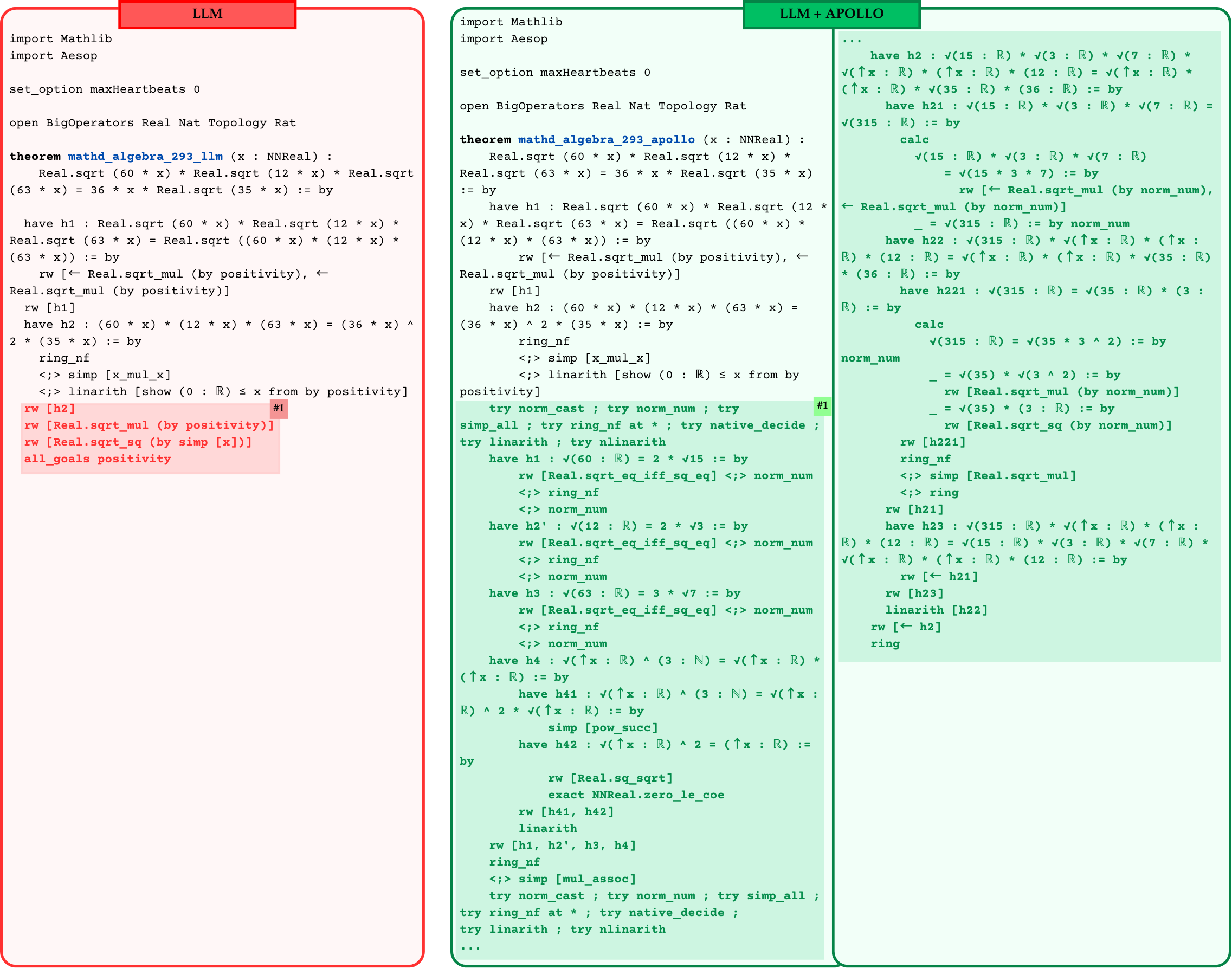
\n ## Code Comparison Diagram: LLM vs. LLM + APOLLO Proof Generation ### Overview The image displays a side-by-side comparison of two Lean 4 code blocks, each contained within a colored, rounded rectangle. The left block, outlined in red, is labeled "LLM". The right block, outlined in green, is labeled "LLM + APOLLO". Both blocks contain formal mathematical proofs for what appears to be the same underlying algebraic theorem, but the proof strategies and lengths differ significantly. The "LLM + APOLLO" proof is substantially longer and more detailed. ### Components/Axes * **Layout:** Two vertical panels. * **Left Panel (LLM):** Red border, light pink background. Header text: "LLM" in a red box. * **Right Panel (LLM + APOLLO):** Green border, light green background. Header text: "LLM + APOLLO" in a green box. * **Content Type:** Formal proof code written in the Lean 4 theorem prover language. * **Language:** The primary language is Lean 4 code. Mathematical notation is embedded within the code (e.g., `√`, `*`, `^`, `:=`). * **Annotations:** The left panel contains a highlighted red section with the comment `#1`. ### Detailed Analysis #### **Left Panel: LLM Proof** **Theorem Name:** `mathd_algebra_293_llm` **Goal:** Prove that for `x : NNReal`, `Real.sqrt (60 * x) * Real.sqrt (12 * x) * Real.sqrt (63 * x) = 36 * x * Real.sqrt (35 * x)`. **Proof Structure (Transcribed):** ```lean import Mathlib import Aesop set_option maxHeartbeats 0 open BigOperators Real Nat Topology Rat theorem mathd_algebra_293_llm (x : NNReal) : Real.sqrt (60 * x) * Real.sqrt (12 * x) * Real.sqrt (63 * x) = 36 * x * Real.sqrt (35 * x) := by have h1 : Real.sqrt (60 * x) * Real.sqrt (12 * x) * Real.sqrt (63 * x) = Real.sqrt ((60 * x) * (12 * x) * (63 * x)) := by rw [← Real.sqrt_mul (by positivity), ← Real.sqrt_mul (by positivity)] rw [h1] have h2 : (60 * x) * (12 * x) * (63 * x) = (36 * x) ^ 2 * (35 * x) := by ring_nf <;> simp [x_mul_x] <;> linarith [show (0 : ℝ) ≤ x from by positivity] rw [h2] -- #1 rw [Real.sqrt_mul (by positivity)] rw [Real.sqrt_sq (by simp [x])] all_goals positivity ``` * **Key Steps:** The proof uses a `have` tactic to assert an intermediate equality `h1` by combining square roots. It then rewrites using `h1` and asserts a second equality `h2` about the product inside the square root. The final steps rewrite using `h2` and simplify the square root of a square. * **Highlighted Section:** The lines from `rw [h2]` to `all_goals positivity` are highlighted in a darker pink/red, with a comment `#1` in the right margin. #### **Right Panel: LLM + APOLLO Proof** **Theorem Name:** `mathd_algebra_293_apollo` **Goal:** Identical to the LLM proof. **Proof Structure (Transcribed - Key Sections):** The proof is much longer. It begins with similar imports and setup, then proceeds with a more granular, step-by-step approach. **Initial Steps (Similar to LLM):** ```lean have h1 : Real.sqrt (60 * x) * Real.sqrt (12 * x) * Real.sqrt (63 * x) = Real.sqrt ((60 * x) * (12 * x) * (63 * x)) := by rw [← Real.sqrt_mul (by positivity), ← Real.sqrt_mul (by positivity)] rw [h1] have h2 : (60 * x) * (12 * x) * (63 * x) = (36 * x) ^ 2 * (35 * x) := by ring_nf <;> simp [x_mul_x] <;> linarith [show (0 : ℝ) ≤ x from by positivity] ``` **Divergence and Elaboration (After `rw [h2]`):** Instead of directly simplifying the square root, the proof enters a long sequence of `try` tactics and then explicitly breaks down the square roots of the numerical coefficients. ```lean try norm_cast ; try norm_num ; try simp_all ; try ring_nf at * ; try native_decide ; try linarith ; try nlinarith have h1 : √(60 : ℝ) = 2 * √15 := by rw [Real.sqrt_eq_iff_sq_eq] <;> norm_num <;> ring_nf <;> norm_num have h2' : √(12 : ℝ) = 2 * √3 := by ... (similar structure) have h3 : √(63 : ℝ) = 3 * √7 := by ... have h4 : √(↑x : ℝ) ^ (3 : ℕ) = √(↑x : ℝ) * (↑x : ℝ) := by ... ``` The proof then continues with a lengthy `calc` block that meticulously shows the equality step-by-step, factoring and recombining the square roots of the prime factors (15, 3, 7) and the variable `x`. It uses lemmas like `h21`, `h22`, `h221`, and `h23` to manage intermediate results. **Final Lines:** ```lean rw [h23] linarith [h22] rw [← h2] ring ``` ### Key Observations 1. **Proof Strategy:** The LLM proof is concise, relying on powerful automation tactics (`ring_nf`, `simp`, `linarith`) to close the goal quickly after asserting the key algebraic identity `h2`. The LLM+APOLLO proof is verbose and explicit, manually decomposing the problem into lemmas about individual square roots and then reconstructing the proof in a `calc` block. 2. **Length and Detail:** The LLM+APOLLO proof is approximately 3-4 times longer in terms of lines of code. 3. **Use of Automation:** The LLM proof uses automation aggressively at the end. The LLM+APOLLO proof uses a block of `try` tactics early on but then proceeds with mostly manual, detailed steps. 4. **Highlighted Region:** The red highlight in the LLM panel draws attention to the final simplification steps, which are the point where the concise automation is applied. ### Interpretation This image is a technical comparison demonstrating two different approaches to automated theorem proving in Lean 4 for the same mathematical statement. * **What it shows:** It contrasts a "standard" LLM-generated proof (left) with a proof generated or augmented by a system called "APOLLO" (right). The LLM proof is efficient and relies on the prover's built-in automation. The APOLLO-augmented proof is more pedagogical and explicit, breaking the problem down into fundamental algebraic steps. * **Relationship between elements:** The side-by-side layout invites direct comparison. The identical theorem statement and initial steps establish a common ground, highlighting the divergence in proof strategy after the key identity `h2` is established. * **Potential Meaning:** The comparison likely aims to showcase a trade-off. The LLM proof is shorter and may be preferred for efficiency. The APOLLO proof, while longer, is more transparent, easier for a human to follow, and may be more robust or generalizable because it avoids relying on the "black box" of powerful automation tactics. The highlighted section in the LLM proof may indicate the specific point where APOLLO's more detailed approach begins. This could be illustrating APOLLO's ability to generate more verifiable, step-by-step proofs compared to an LLM that might take shortcuts via automation.