## Histogram: Distribution of Relative Length Differences
### Overview
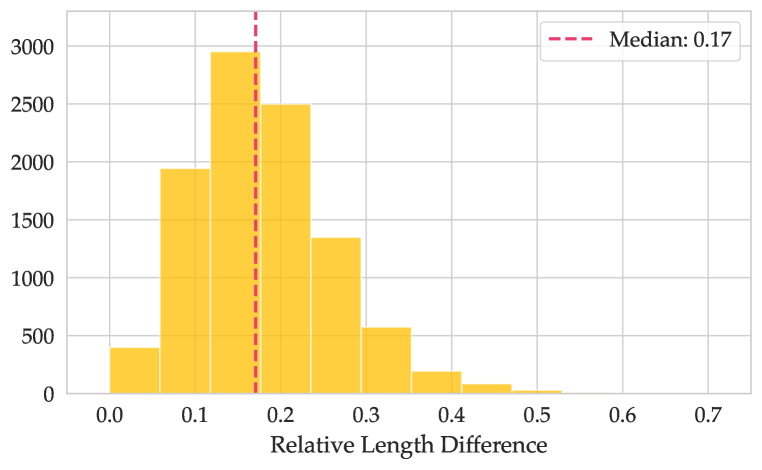
The image displays a histogram visualizing the distribution of "Relative Length Difference" values. The x-axis represents the relative length difference (0.0 to 0.7), and the y-axis represents frequency (0 to 3000). A red dashed line labeled "Median: 0.17" is overlaid on the chart.
### Components/Axes
- **X-axis**: "Relative Length Difference" with tick marks at 0.0, 0.1, 0.2, 0.3, 0.4, 0.5, 0.6, 0.7.
- **Y-axis**: "Frequency" with tick marks at 0, 500, 1000, 1500, 2000, 2500, 3000.
- **Legend**: Located in the top-right corner, indicating the red dashed line corresponds to the median value (0.17).
- **Bars**: Orange-colored histogram bars representing frequency counts.
### Detailed Analysis
- **Bars**:
- **0.0–0.1**: Frequency ~400 (short bar).
- **0.1–0.15**: Frequency ~3000 (tallest bar).
- **0.15–0.2**: Frequency ~2500 (second tallest bar).
- **0.2–0.3**: Frequency ~1400 (moderate bar).
- **0.3–0.4**: Frequency ~600 (smaller bar).
- **0.4–0.5**: Frequency ~200 (very small bar).
- **0.5–0.7**: Frequency ~50 (minimal bar).
- **Median Line**: Red dashed line at x = 0.17, intersecting the histogram near the peak.
### Key Observations
1. **Peak Distribution**: The highest frequency (~3000) occurs between 0.1 and 0.15, indicating the most common relative length differences fall in this range.
2. **Median Position**: The median (0.17) is slightly right of the peak, suggesting a right-skewed distribution.
3. **Rapid Decline**: Frequencies drop sharply after 0.2, with minimal counts beyond 0.4.
4. **Skewness**: The distribution is asymmetric, with a long tail extending toward higher relative length differences.
### Interpretation
The data suggests that most relative length differences cluster around 0.1–0.2, with the median (0.17) reflecting the central tendency. The right skew implies that while most values are concentrated in the lower range, a subset of measurements exhibits larger discrepancies. This could indicate variability in a process or system being measured, such as manufacturing tolerances or biological measurements. The sharp decline after 0.2 suggests that extreme values are rare, but their presence may warrant further investigation into outliers or measurement errors.