TECHNICAL ASSET FINGERPRINT
484f446859734853c6cb5f59
Click to view fullscreen
Press ESC or click to close
FOUND IN PAPERS
EXPERT: gemini-2.0-flash VERSION 1
RUNTIME: nugit/gemini/gemini-2.0-flash
INTEL_VERIFIED
## Line Charts: Algorithm Performance vs. Number of Variables
### Overview
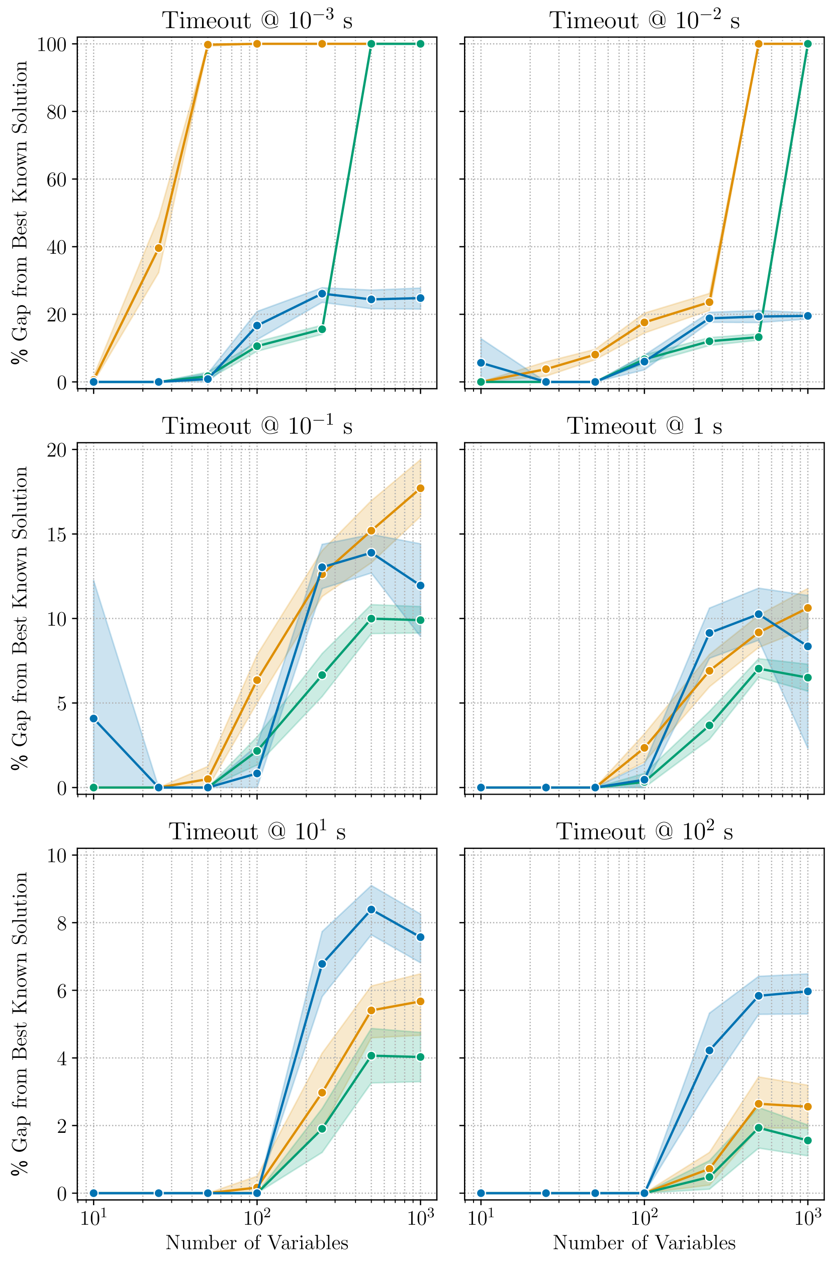
The image contains six line charts arranged in a 2x3 grid. Each chart displays the performance of three algorithms (represented by blue, orange, and green lines) as a function of the number of variables. Performance is measured as the "% Gap from Best Known Solution". Each chart corresponds to a different timeout value, ranging from 10^-3 seconds to 10^2 seconds. The x-axis (Number of Variables) is logarithmic, spanning from 10^1 to 10^3. Shaded regions around each line represent uncertainty or variability in the algorithm's performance.
### Components/Axes
* **X-axis (Horizontal):** "Number of Variables". Logarithmic scale with markers at 10^1, 10^2, and 10^3.
* **Y-axis (Vertical):** "% Gap from Best Known Solution". Linear scale, with the range varying across the charts.
* Top row: 0 to 100
* Middle row: 0 to 20
* Bottom row: 0 to 10
* **Titles:** Each chart has a title indicating the timeout value: "Timeout @ 10^-3 s", "Timeout @ 10^-2 s", "Timeout @ 10^-1 s", "Timeout @ 1 s", "Timeout @ 10^1 s", "Timeout @ 10^2 s".
* **Data Series:** Three data series are plotted on each chart, represented by colored lines with circular markers. The colors are blue, orange, and green. There is no explicit legend, but the colors are consistent across all charts.
* **Grid:** Each chart has a grid to aid in reading values.
### Detailed Analysis
**Chart 1: Timeout @ 10^-3 s (Top-Left)**
* **Blue Line:** Starts at 0% gap for 10^1 variables, remains at 0% until approximately 10^2 variables, then increases to approximately 25% gap and remains relatively constant.
* **Orange Line:** Starts at 0% gap for 10^1 variables, increases sharply to 40% gap at approximately 30 variables, then increases sharply again to 100% gap at approximately 10^2 variables, and remains constant.
* **Green Line:** Starts at 0% gap for 10^1 variables, remains at 0% until approximately 10^2 variables, then increases sharply to 100% gap and remains constant.
**Chart 2: Timeout @ 10^-2 s (Top-Right)**
* **Blue Line:** Starts at 0% gap for 10^1 variables, remains at 0% until approximately 50 variables, then increases to approximately 15% gap and remains relatively constant.
* **Orange Line:** Starts at 0% gap for 10^1 variables, increases to approximately 10% gap at approximately 50 variables, then increases sharply again to 100% gap at approximately 10^2 variables, and remains constant.
* **Green Line:** Starts at 0% gap for 10^1 variables, remains at 0% until approximately 10^2 variables, then increases sharply to 100% gap and remains constant.
**Chart 3: Timeout @ 10^-1 s (Middle-Left)**
* **Blue Line:** Starts at approximately 4% gap for 10^1 variables, decreases to 0% at approximately 30 variables, then increases to approximately 14% gap at approximately 10^2 variables, and then decreases to approximately 12% gap at 10^3 variables.
* **Orange Line:** Starts at 0% gap for 10^1 variables, increases to approximately 17% gap at approximately 10^2 variables, and then increases to approximately 18% gap at 10^3 variables.
* **Green Line:** Starts at 0% gap for 10^1 variables, increases to approximately 10% gap at approximately 10^2 variables, and then remains relatively constant.
**Chart 4: Timeout @ 1 s (Middle-Right)**
* **Blue Line:** Starts at 0% gap for 10^1 variables, remains at 0% until approximately 10^2 variables, then increases to approximately 8% gap at approximately 300 variables, and then decreases to approximately 6% gap at 10^3 variables.
* **Orange Line:** Starts at 0% gap for 10^1 variables, increases to approximately 6% gap at approximately 10^2 variables, and then increases to approximately 10% gap at 10^3 variables.
* **Green Line:** Starts at 0% gap for 10^1 variables, increases to approximately 4% gap at approximately 10^2 variables, and then increases to approximately 7% gap at 10^3 variables.
**Chart 5: Timeout @ 10^1 s (Bottom-Left)**
* **Blue Line:** Starts at 0% gap for 10^1 variables, remains at 0% until approximately 10^2 variables, then increases to approximately 8% gap at approximately 300 variables, and then decreases to approximately 7% gap at 10^3 variables.
* **Orange Line:** Starts at 0% gap for 10^1 variables, increases to approximately 5% gap at approximately 10^3 variables.
* **Green Line:** Starts at 0% gap for 10^1 variables, increases to approximately 4% gap at approximately 10^3 variables.
**Chart 6: Timeout @ 10^2 s (Bottom-Right)**
* **Blue Line:** Starts at 0% gap for 10^1 variables, remains at 0% until approximately 10^2 variables, then increases to approximately 6% gap at approximately 10^3 variables.
* **Orange Line:** Starts at 0% gap for 10^1 variables, remains at 0% until approximately 10^2 variables, then increases to approximately 3% gap at approximately 10^3 variables.
* **Green Line:** Starts at 0% gap for 10^1 variables, remains at 0% until approximately 10^2 variables, then increases to approximately 2% gap at approximately 10^3 variables.
### Key Observations
* For very short timeouts (10^-3 s and 10^-2 s), the orange and green algorithms quickly reach a 100% gap from the best known solution as the number of variables increases. The blue algorithm performs better, maintaining a lower gap.
* As the timeout increases, the performance of all three algorithms improves, with the gap from the best known solution generally decreasing.
* The blue algorithm tends to perform better than the orange and green algorithms, especially for shorter timeouts.
* The shaded regions indicate variability in the algorithm performance, which tends to be larger for shorter timeouts and smaller numbers of variables.
### Interpretation
The charts illustrate the trade-off between timeout duration and solution quality for three different algorithms. The data suggests that:
* **Timeout Matters:** Increasing the timeout generally leads to better solutions (smaller gap from the best known solution).
* **Algorithm Choice is Critical:** The choice of algorithm significantly impacts performance, especially when the timeout is limited. The blue algorithm appears to be more robust and provides better solutions within shorter timeframes.
* **Problem Complexity:** As the number of variables increases, the problem becomes more complex, and the algorithms require more time to find good solutions. This is evident in the increasing gap from the best known solution for shorter timeouts.
* **Variability:** The shaded regions highlight the variability in the algorithm performance. This variability could be due to factors such as the specific problem instance, the starting point of the algorithm, or random fluctuations in the search process.
The data demonstrates that selecting an appropriate algorithm and allowing sufficient timeout are crucial for achieving good solutions, especially for complex problems with a large number of variables.
DECODING INTELLIGENCE...